Building Aligned Intelligence System. Part I: Creating GPT Assistant

In recent years, the field of natural language processing has witnessed a remarkable breakthrough with the advent of Large Language Models (LLMs). These models have demonstrated unprecedented performance in a wide range of language tasks, from text generation to question answering. However, the mathematical formulation of these models and the techniques used to fine-tune them for specific tasks can be complex and daunting for many researchers and practitioners. In this post, we will delve into the mathematical underpinnings of LLMs, with a focus on ChatGPT and parameter efficient fine-tuning. We will explore the key concepts and techniques involved in these models, and provide a comprehensive guide to help you understand and apply them in your own research and development. So, whether you’re a seasoned NLP expert or just starting out, join us on this journey to unlock the secrets of LLMs and take your NLP skills to the next level.

‘Engaging preamble’ generated by ChatGPT.

There will be two blogposts. The first post will be helpful to those who want to become acquainted with the RLHF pipeline as it focuses on InstructGPT/ChatGPT development. The second one is for those who are interested in applying large language models to specific tasks.

Here is the partial list of the sources I used for this and the following parts:

• Papers:
  • Scalable agent alignment via reward modeling: a research direction (Leike et al., 2018)
  • Language Models are Few-Shot Learners (Brown et al., 2020)
  • Fine-Tuning Language Models from Human Preferences (Ziegler et al., 2020)
  • Training language models to follow instructions with human feedback (Ouyang et al., 2022)
  • Learning to summarize from human feedback (Stiennon et al., 2022)
  • Training a Helpful and Harmless Assistant with Reinforcement Learning from Human Feedback (Bai et al., 2022)
  • Deep Reinforcement Learning from Human Preferences (Christiano et al., 2023)
  • Scaling Down to Scale Up: A Guide to Parameter-Efficient Fine-Tuning (Lialin et al., 2023)
  • Chain-of-Thought Prompting Elicits Reasoning in Large Language Models (Wei et al., 2023)
• Posts:
  • RLHF: Reinforcement Learning from Human Feedback (Chip Huyen, 2023)
  • Illustrating Reinforcement Learning from Human Feedback (RLHF) (Lambert et al., 2022)
  • Prompt Engineering (Lilian Weng, 2023)
  • OpenAI GPT Models (Lei Mao, 2023)
  • Techniques to improve reliability (OpenAI, 2023)

GPT assistant building pipeline can be divided into 4 stages, each of which will be described here, starting from an overview of transformer architecture.

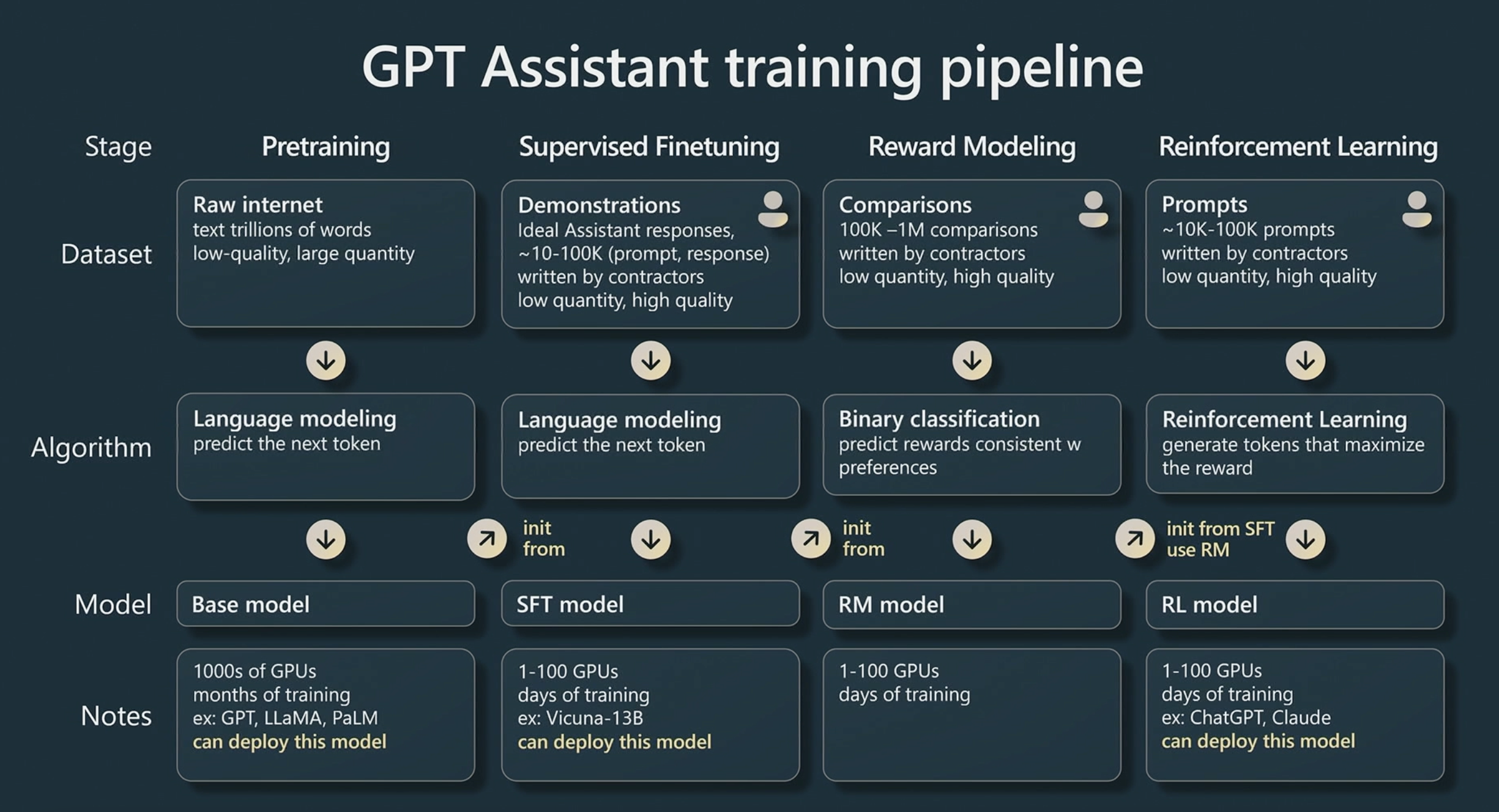A diagram from Andrej Karpathy talk illustrating the four steps of GPT assistant training pipeline: (1) base model pretraining, (2) supervised fine-tuning (SFT), (3) reward model (RM) training, and (4) reinforcement learning via policy optimization on this reward model and human feedback (RLHF).

Pretraining Base model

Language modelling

In 2018 OpenAI presented Generative pre-trained transformer (GPT), a type of deep learning model, that is designed to generate natural language text. Their work, which they humbly called Improving Language Understanding by Generative Pre-Training, along with famous Attention is all you need paper, gave birth to the entire family of large language models and changed an entire AI industry in just 5 years.

The model was trained on a large corpus of text data with a completion task. During such training model is fed by a partial sequence of words, called prompt or context vector of tokens, and then asked to generate a response to complete that prompt. The model learns to predict the probability of the next token $x_{k+1}$ in a sequence given by previous tokens $x = (x_1, \dots x_k)$ sampled from dataset $\mathcal{D}$. Strictly speaking, we search for parameters of neural network $\phi$, such that they minimize the cross-entropy loss

\[\mathcal{L}(\phi) = -\mathbb{E}_{x \sim \mathcal{D}}[\log \pi_\phi(x_{k+1} \mid x_1, \dots, x_{k})],\]

where $\pi_\phi$ is a language model output.

Though GPT-1 was pre-trained as an autoregressive language model, transformer’s fine-tuning and inference didn’t have to be autoregressive and language model could be further fine-tuned for specialized natural language processing tasks.

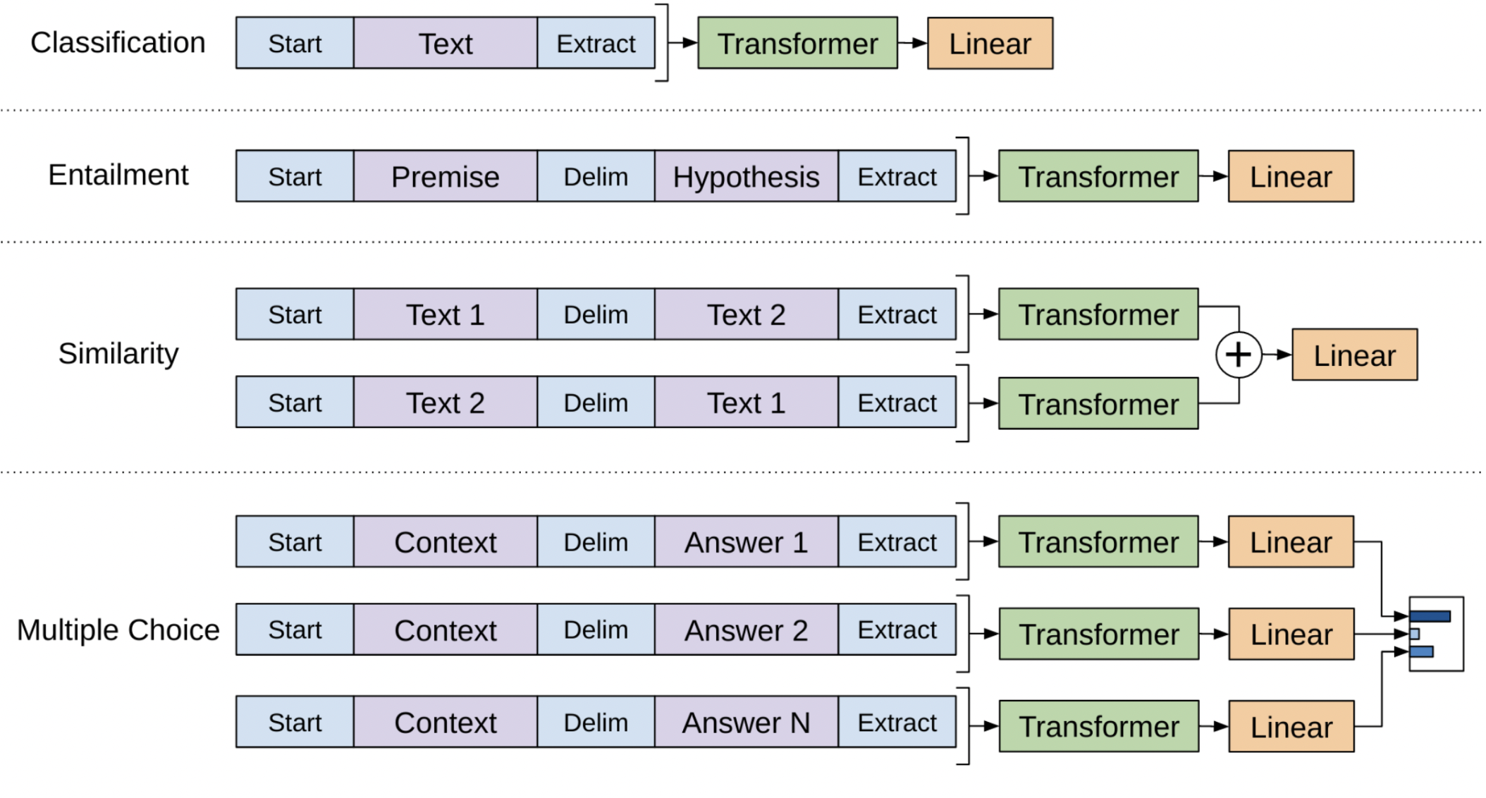Input transformations for fine-tuning GPT on different tasks.

The major conclusion from this paper was that it is no longer necessary to develop specific neural network architectures for specific natural language processing tasks. Transfer learning from GPT language model pre-trained with large corpus of text data was already sufficient.

Transformer architecture

The process of text generation with GPT is the following. First, embedding layer takes sequence of tokens $x$ and outputs

\[h_0 = x \mathbf{W_e} + \mathbf{W_p},\]

where $\mathbf{W_e}$ and $\mathbf{W_p}$ are token and position embedding matrices respectively. Then these embedding vectors are processed by so-called transformer, consisting of multiple transformer blocks (more about it later):

\[h_n = \operatorname{Transformer-block}(h_{n-1}) \quad n = 1, \dots, N.\]

And finally we get the token output distribution by taking $h_N$ and run it through unembedding layer and softmax function:

\[\pi_\phi(\cdot \mid x) = \operatorname{softmax}(h_N \mathbf{W_e}^T).\]

Simplified view of GPT architecture. Recently other techniques to encode token positions have appeared, such as Rotary Position Embeddings (RoPE) and Attention with Linear Biases (ALiBi). They are out of the scope of this post

The key innovation of GPT is its use of a transformer architecture, which allows the model to process long sequences of text efficiently. This makes GPT particularly well-suited for tasks that require generating long, coherent pieces of text, such as writing articles or answering questions. The core of the transformer is a scaled dot product attention operation, which takes as input a set of queries $\mathbf{Q}$, keys $\mathbf{K}$ and values $\mathbf{V}$ and outputs

\[\operatorname{Attention}(\mathbf{Q}, \mathbf{K}, \mathbf{V}) = \operatorname{softmax} \Big( \frac{\mathbf{QK}^T}{\sqrt{d}} \Big) \cdot \mathbf{V},\]

where $d$ is a hidden dimensionality for queries and keys. The goal is to have an attention mechanism with which any element in a sequence can attend to any other while still being efficient to compute.

Transformer architecture can be one of two types: encoder or decoder. The only difference between the two is whether mask is applied to attention layer. This modification in decoder architecture is crucial for next-token-prediction task, because it prevents positions from attending to subsequent positions attention layer modified by mask. Combined with the fact that the output embeddings are offset by one position, masking ensures that the predictions for position $i$ can depend only on the known outputs at positions less than $i$. It can be implemented inside of scaled dot-product attention by masking out (setting to $-\infty$) all values in the $\mathbf{QK}^T$ matrix which correspond to illegal connections.

The scaled dot product attention allows a network to attend over a sequence. However, often there are multiple different aspects a sequence element wants to attend to, and a single weighted average is not a good option for it. The attention mechanism can be extended to multiple heads, i.e. multiple different query-key-value triplets on the same features. Specifically, given $\mathbf{Q}$, $\mathbf{K}$, and $\mathbf{V}$ matrices, we transform those into $k$ sub-queries, sub-keys, and sub-values, respectively, which we run through the scaled dot product attention independently. Afterward, we concatenate the heads and combine them with a final weight matrix $\mathbf{W}^O$. Mathematically, we can express this operation as:

\[\operatorname{MultiHead}(\mathbf{Q}, \mathbf{K}, \mathbf{V})=[\operatorname{head}_1; \dots; \operatorname{head}_k] \cdot \mathbf{W}^O,\]

where

\[\operatorname{head}_i = \operatorname{Attention}(\mathbf{QW}_i^Q, \mathbf{KW}_i^W, \mathbf{VW}_i^V), \quad i = 1, \dots, k.\]

We’ll refer to this as multi-head attention layer with the learnable parameters $\mathbf{W}^Q_{1 \dots k}, \mathbf{W}^K_{1 \dots k}, \mathbf{W}^V_{1 \dots k}$ and $\mathbf{W}^O$ (also called multi-head self-attention for $\mathbf{Q} = \mathbf{K} = \mathbf{V}$). Such mechanism allows the model to jointly attend to information from different representation subspaces at different positions. The output of multi-head attention is added to the original input using a residual connection, and we apply a consecutive layer normalization on the sum.

Transformer is basically a stack of $N$ identical blocks with multi-head attention. In addition to attention sub-layers, each block contains a fully connected feed-forward network, which is applied to each position separately and identically. This consists of two linear transformations with a nonlinear function in between, e.g. ReLU¹:

\[\operatorname{FFN}(x) = \max(0, x\mathbf{W}_1)\mathbf{W}_2\]

After feed forward block residual connection with normalization layer is added again.

Generative pre-trained transformer decoder architecture. In some recent implementations one can find layer normalization being applied to input stream of the submodules (right before multi-head attention and feed forward layers, not after).

There are many guides on the internet for implementing a transformer. To get more detailed explanations one can follow this tutorial on PyTorch or this one on Jax.

It turned out that the transformer architecture is highly scalable, meaning that it is able to handle large amounts of data and perform well on tasks of varying complexity. It has been shown to achieve SoTA performance on a variety of NLP benchmarks, demonstrating its ability to scale to handle complex tasks and large datasets. GPT-1 was just a starting point and later OpenAI presented much bigger models, such as GPT-2 and GPT-3. Here is a table for comparison:

Model	Train data size	Transformer blocks	Context size	Total parameters
GPT-1	20M tokens	12	512 tokens	117M
GPT-2	9B tokens	48	1024 tokens	1.5B
GPT-3	300B tokens	96	2048 tokens	175B

There is no official information yet on how large GPT-4 is, but there’ve been some rumors that it consists of multiple expert models with 220B parameters.

Language modelling is by far the most resource-intensive phase in InstructGPT training. According to OpenAI the rest of their pipeline used less than 2% of the compute and data relative to model pretraining. One way of thinking about this process is that at the end of this phase base LLM already has all the required capabilities, but they are difficult to elicit and the rest of the process is aimed to “unlock” them.

Supervised fine-tuning (SFT) for dialogue

Suppose we have a pretrained large language model. But this model is far from being a useful assistant. It doesn’t answer questions, it only wants to complete internet documents. Chip Huyen provided a good example in her blogpost: if you give the pretrained model a question, say, How to make pizza, any of the following could be valid completion.

• Adding more context to the question: for a family of six
• Adding follow-up questions: ? What ingredients do I need? How much time would it take?
• Actually giving the answer

The third option is preferred if you’re looking for an answer. In order to achieve it, base model can be tricked into performing tasks with prompt engineering. For example, we can give model an instruction and expect it to follow, e.g.:

Classify the text into neutral, negative or positive. 
Text: I think the vacation is okay.
Sentiment:

Output:

Neutral

This is an example of zero-shot prompting. One can also give a few demonstration examples of how the dialogue should look like and expect the model to continue in the same vein. This is called few-shot prompting.

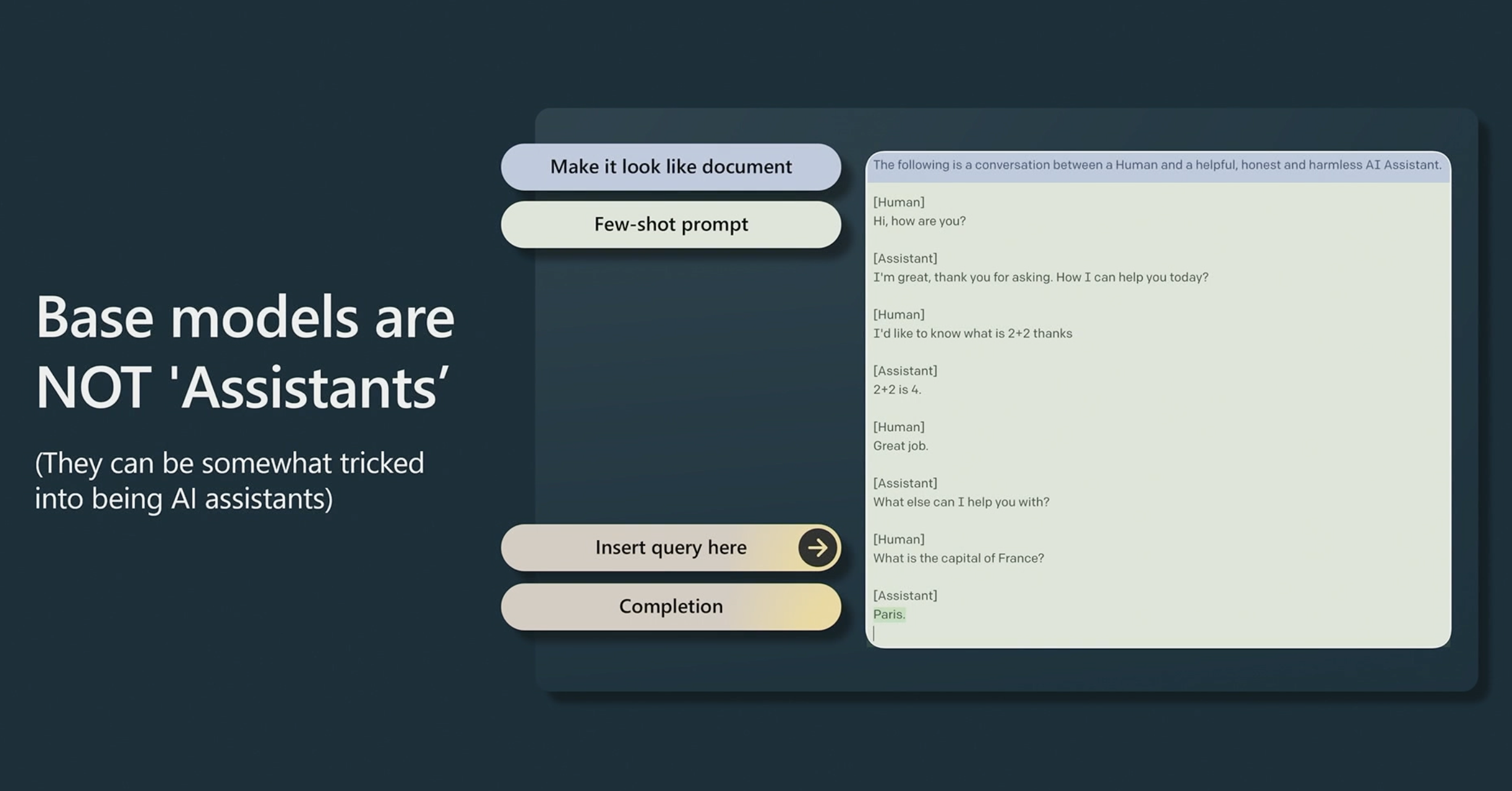Few-shot prompt engineering example from Andrej Karpathy talk

Standard few-shot prompting works well for many tasks but is still not a perfect technique. A more efficient way is to train the model to answer questions directly. This is what SFT does: its goal is to optimize the pretrained model to generate the responses that users are looking for. At this stage labelers provide demonstrations of the desired behaviour on the input prompt distribution. Then a pretrained model is fine-tuned on this data learning to appropriately respond to prompts of different use cases (e.g. question answering, summarization, translation).

Supervised fine-tuning stage of InstructGPT pipeline.

Basically, SFT model is an initial language model for RLHF. For InstructGPT training OpenAI fine-tuned three different versions of GPT-3 (1.3B, 6B and 175B) on labeler-written demonstration prompts. OpenAI called supervised finetuning behavior cloning: we demonstrate how the model should behave, and the model clones this behavior. Anthropic, for example, used a different technique: they trained their SFT model by distilling an original language model on context clues for their “helpful, honest, and harmless” criteria.

Reward Model (RM) training

The problem with SFT is that model learns what kind of responses are plausible for a given context, but it receives no information on how good or bad a response is. At the same time while it is easy for humans to understand which sentences are better than others, it is difficult to formulate and automate reasons for their choice.

This is where human feedback (HF) comes into play. At this stage datasets of comparisons between model outputs is collected: annotators indicate which output of SFT model they prefer for a given input. At first glance, it may seem that labelers must apply a scalar score directly to each output in order to create data for reward model, but this is difficult to do in practice. The differing values of humans cause these scores to be uncalibrated and noisy. Instead, rankings are used to compare the outputs of multiple models and create a much better regularized dataset.

To collect ranking data, human labelers are presented with $K_x$ generated samples conditioned on the same prompt $x$ (in InstructGPT paper, $K_x$ is anywhere between $4$ and $9$). This produces

\[\binom{K_x}{2} = \frac{K_x(K_x-1)}{2}\]

comparisons for each prompt. Labelers express preferences for one answer, denoted as $y_w \succ y_l \mid x$ with $y_w$ being a preferred answer over $y_l$.

Then a preference model is trained to predict the human-preferred output. Starting from the SFT model with the final unembedding layer removed, a reward model $r_\theta(x, y)$ is trained to take in a prompt $x$ and response $y$, and output a scalar reward $r$. OpenAI used 6B RM with to evaluate 175B language model as they found out that while larger RM had the potential to achieve lower validation loss, their training was more unstable and using a 175B RM and value function greatly increase the compute requirements of reinforcement learning. Deepmind, on a contrary, trained Chinchilla models with 70B parameters for both reward and language model. An intuition would be that reward models need to have similar capacity to understand the text given to them as a model would need in order to generate said text.

Reward modelling stage of InstructGPT pipeline. Boxes A-D are samples from the SFT model that get ranked by labelers

There are a number of approaches used to model preferences, the Bradley-Terry model being a popular choice:

\[\mathbb{P}(y_i \succ y_j \mid x) = \frac{\exp(r_\theta(x, y_i))}{\exp(r_\theta(x, y_i))+\exp(r_\theta(x, y_j))}.\]

Framing the problem as a balanced binary classification we come up to the negative log-likelihood loss:

\[\mathcal{L}(\theta) = -\mathbb{E}_{(x, y_w, y_l) \sim \mathcal{D}}\bigg[\frac{1}{\binom{K_x}{2}}\log \sigma (r_\theta(x, y_w) - r_\theta(x, y_l))\bigg].\]

This way model learns to maximize the difference between rewards for chosen and rewards for rejected answers. At the end of training, the reward model is normalized so that

\[\mathbb{E}_{(x, y) \sim \mathcal{D}}[r_\theta(x, y)]=0\]

for all $x$.

The success of reward modeling relies heavily on the quality of the reward model. If the reward model only captures most aspects of the objective but not all of it, this can lead the agent to find undesirable degenerate solutions. In other words, the agent’s behavior depends on the reward model in a way that is potentially very fragile.

Reinforcement Learning with Human Feedback (RLHF)

At final stage output of the reward model used as a scalar reward to optimize a policy. Following Stiennon et al. (2020), authors of InstructGPT fine-tuned the SFT model on their environment using on-policy algorithm, called Proximal Policy Optimization (PPO), Schulman et al. (2017). The environment is a bandit environment which presents a random customer prompt to language model and expects a response to the prompt with a sequence of probability distributions over tokens $\pi(y \mid x)$. The action space of this policy is all the tokens corresponding to the vocabulary of the language model and the observation space is the distribution of possible input token sequences.

Given the prompt and response, environment produces a reward determined by RM and ends the episode.

Policy optimization stage of InstructGPT pipeline.

A per-token KL penalty is added to mitigate overoptimization of the reward model. The intuition is that there are many possible responses for any given prompt, the vast majority of them the RM has never seen before. For many of those unknown $(x, y)$ pairs, the RM might give an extremely high or low score by mistake. Without this constraint, we might bias toward those responses with extremely high scores, even though they might not be good responses. The following modified reward function in RL training is maximized:

\[\begin{aligned} \mathcal{J}_{\operatorname{PPO}}(\phi) &=\mathbb{E}_{(x,y)\sim \mathcal{D}_{\pi_\phi^{\operatorname{RL}}}}\big[r_\theta(x,y)\big]-\beta D_{\operatorname{KL}}(\pi_\phi^{\operatorname{RL}} \mid \mid \pi^{\operatorname{SFT}}) \\ &= \mathbb{E}_{(x,y)\sim \mathcal{D}_{\pi_\phi^{\operatorname{RL}}}}\Big[r_\theta(x,y)-\beta \log \frac{\pi_\phi^{\operatorname{RL}}(y \mid x)}{\pi^{\operatorname{SFT}}(y \mid x)}\Big], \end{aligned}\]

where $\pi_\phi^{\operatorname{RL}}$ is the learned RL policy, $\pi^{\operatorname{SFT}}$ is the supervised trained model. The KL-divergence coefficient, $\beta$ controls the strength of the KL penalty. InstructGPT authors also experimented with mixing the pretraining gradients into the PPO gradients, in order to fix the performance regressions on public NLP datasets. They called these models “PPO-ptx”:

\[\mathcal{J}_{\operatorname{PPO-ptx}}(\phi) = \mathcal{J}_{\operatorname{PPO}}(\phi) + \gamma \mathbb{E}_{x \sim \mathcal{D}_{\operatorname{pretrain}}}[\log\pi_\phi^{\operatorname{RL}}(x)],\]

where $D_{\operatorname{pretrain}}$ is the pretraining distribution. The pretraining loss coefficient $\gamma$ controls strength of pretraining gradients.

At this stage one has to be careful to avoid reward hacking - an effect that lets the agent get more reward than intended by exploiting loopholes in the process determining the reward. An agent can exploit some misspecification in the reward function, e.g. when the reward function incorrectly provides high reward to some undesired behavior. One potential source for such exploit is the reward model’s vulnerability to adversarial inputs. The agent might figure out how to specifically craft these adversarially perturbed inputs in order to trick the reward model into providing higher reward than the user intends.

Finally, RM stage and RL stage can be iterated continuously: collect more comparison data on the current best policy, then use it to train a new RM and then a new policy. In InstructGPT pipeline, most of comparison data comes from supervised policies, with some coming from PPO policies.

Details of RL algorithm

Consider response generation as a sequence of input states and actions. Let’s denote input state at timestep $t$ as

\[s_t=(x, y_1, \dots y_{t-1}),\]

where $y_s$ is a response token, generated at timestep $s$ by actor $\pi_\phi$. During rollout at each timestep $t$ RL model is penalized by

\[R_{t+1} = -\beta \log \frac{\pi_\phi^{\operatorname{RL}}(y_t \mid s_t)}{\pi^{\operatorname{SFT}}(y_t \mid s_t)}\]

until it reaches terminal state and receives final reward

\[R_T = r_\theta(x, y)-\beta \log \frac{\pi_\phi^{\operatorname{RL}}(y_{T-1} \mid s_t)}{\pi^{\operatorname{SFT}}(y_{T-1} \mid s_t)}.\]

Backup diagram illustrating one step of sequence generation in terms of reinforcement learning

In general we are interested in maximizing return, which is a total sum of rewards going forward:

\[G_t = R_{t+1} + R_{t+2} + \dots + R_T.\]

It is also common to use the discounted return:

\[G_t = R_{t+1} + \gamma R_{t+2} + \dots + \gamma^{T-t} R_T = \sum_{k=0}^{T-t-1} \gamma^k R_{t+k+1},\]

where the discounting factor $\gamma \in [0, 1]$ trades off later rewards to earlier ones.

Besides actor model, we must have a critic $V_\theta(s_t)$, which estimates $G_t$ and is trained with mean-squared loss:

\[\mathcal{L}_V(\theta) = \mathbb{E}_t[(V_\theta(s_t) - G_t)^2]\]

While actor is initialized from SFT model, critic can also be initialized from RM model. With critic network estimating the return under current policy actor network learns to maximize the probability of getting a positive advantage, the relative value of selected response token:

\[\hat{A}_t = G_t - V_\theta(s_t).\]

The equality above² can be used for return calculation, but such estimator would have low bias but high variance. Usually returns and advantages are estimated with a technique called bootstrapping, e.g. with generalized version of advantage estimation (GAE), popularized by Schulman et. al (2018):

\[\begin{aligned} \hat{A}_t = \delta_t + (\gamma \lambda) \delta_{t+1} + \dots = \sum_{k=0}^{T-t-1} (\gamma \lambda)^k \delta_{t+k}, \\ \text{where } \delta_t = R_{t+1} + \gamma V_\theta(s_{t+1}) - V_\theta(s_t) \end{aligned}\]

and $\lambda \in [0,1]$ is a decay factor, penalizing high variance estimates. I recommend this nice post to grasp the idea of GAE.

To train actor network vanilla policy gradient loss can be used:

\[\mathcal{L}^{\operatorname{PG}}(\phi) = -\mathbb{E}_t[\log \pi_\phi(y_t \mid s_t) \hat{A}_t].\]

This way, when $\hat{A}_t$ is positive, meaning that the action agent took resulted in a better than average return, we increase the probability of selecting it again in the future. On the other hand, if an advantage is negative, we reduce the likelihood of selected action.

However, consider the case of optimizing target policy $\pi_\phi$, when the behaviour policy $\pi_{\phi_{\text{old}}}$ is used for collecting trajectories with $\phi_{\text{old}}$ policy parameters before the update. In an original PPO paper it is stated, that while it is appealing to perform multiple steps of optimization on this loss using the same trajectory, doing so is not well-justified, and empirically it often leads to destructively large policy updates. In other words, we have to impose the constraint which won’t allow our new policy to move too far away from an old one. Let $\rho_t(\phi)$ denote the probability ratio between target and behaviour policies:

\[\rho_t(\phi) = \frac{\pi_\phi(y_t \mid x)}{\pi_{\phi_{\operatorname{old}}}(y_t \mid x)},\]

so $\rho_t(\phi_{\operatorname{old}}) = 1$. Then we can minimize the surrogate objective function (the superscript CPI refers to conservative policy iteration)

\[\mathcal{L}^{\text{CPI}}(\phi) = -\mathbb{E}_t[\rho_t(\phi) \hat{A}_t].\]

Indeed,

\[\begin{aligned} \nabla_\phi\mathcal{L}^{\operatorname{PG}}(\phi) \big \vert_{\phi_{\text{old}}} &= -\mathbb{E}_t\big[\nabla_\phi\log \pi_\phi(y_t \mid x)\big \vert_{\phi_{\text{old}}} \hat{A}_t\big] \\ &=-\mathbb{E}_t\bigg[\frac{\nabla_\phi \pi_\phi(y_t \mid s_t) \big \vert_{\phi_{\text{old}}}}{\pi_{\phi_{\text{old}}}(y_t \mid s_t)} \hat{A}_t\bigg] \\ &= -\mathbb{E}_t\big[\nabla_\phi \rho_t(\phi) \big \vert_{\phi_{\text{old}}} \hat{A}_t\big] \\ &= \nabla_\phi\mathcal{L}^{\text{CPI}}(\phi). \end{aligned}\]

Now, we would like to insert the aforementioned constraint into this loss function. The main objective which authors of PPO propose is the following.

\[\mathcal{L}^{\text{CLIP}}(\phi) = -\mathbb{E}_t\Big[\min \big(\rho_t(\phi) \hat{A}_t, \text{clip}(\rho_t(\phi), 1-\epsilon, 1+\epsilon)\hat{A}_t\big)\Big],\]

where $\epsilon$ is a clip ratio hyperparameter. The first term inside $\min$ function, $\rho_t(\phi) \hat{A}_t$ is a normal policy gradient objective. And the second one is its clipped version, which doesn’t allow us to destroy our current policy based on a single estimate, because the value of $\hat{A}_t$ is noisy (as it is based on an output of our network).

The total objective is a combination of clipped loss and error term on the value estimation

\[\mathcal{L}(\phi, \theta) = \mathcal{L}^{\text{CLIP}}(\phi) + c\mathcal{L}_V(\theta).\]

import jax
import jax.numpy as jnp

# actor - policy neural network
# params - learnable parameters
# states[B] - batch of input states
# token_ids[B] - generated response token indices
# advantages[B] - batch of estimated advantages
# logp_old[B] - log-probabilities of generated tokens according to behaviour policy
# eps - clip ratio, usually around 0.2

@jax.jit
def actor_loss(actor, params, states, token_ids, advantages, logp_old, eps=0.2):
    logp_dist = actor.apply(params, states)
    logp = jnp.stack([lp[y] for lp, y in zip(logp_dist, token_ids)])
    ratio = jnp.exp(logp - logp_old)
    clip_adv = jnp.clip(ratio, 1 - eps, 1 + eps) * advantages
    return -jnp.min(ratio * advantages, clip_adv)
    
# critic - value prediction neural network
# returns[B] - batch of discounted returns

@jax.jit
def critic_loss(critic, params, states, returns):
    values = critic.apply(params, states)
    return (values - returns) ** 2

Note on KL approximations

John Schulman, author of PPO algorithm, proposes different estimators of KL-divergence $D_{\operatorname{KL}}(\pi’ \mid \mid \pi)$ in his blogpost. Let $\kappa=\frac{\pi(x)}{\pi’(x)}$, then for $\pi \approx \pi’$ we get empirically:

	Estimation	Bias	Variance
$k_1$	$-\log \kappa$	$0$	High
$k_2$	$\frac{1}{2}(\log \kappa)^2$	Low	Low
$k_3$	$(\kappa-1)-\log \kappa$	$0$	Low

The main advantage of $k_2$ and $k_3$ estimators is the zero probability of getting negative values. Although, with true KL-divergence between $\pi$ and $\pi’$ getting larger we can observe that bias for $k_2$ and variance for $k_3$ are increasing as well.

GPT chatbot limitations

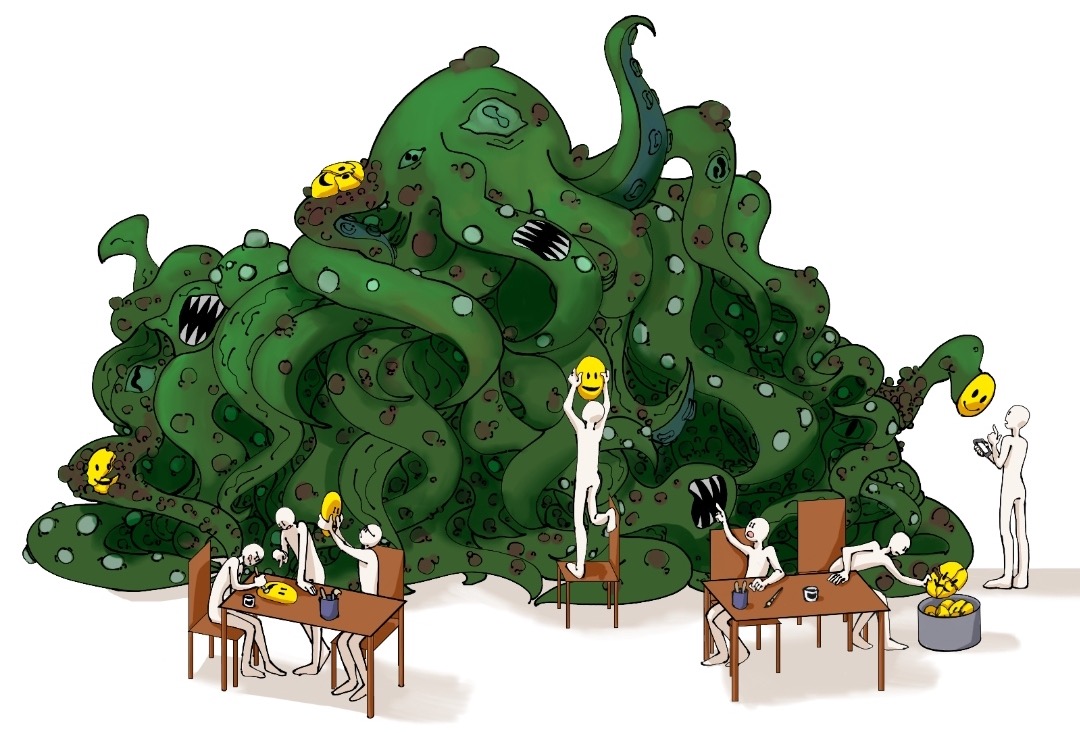Is RLHF just putting smileys on a shoggoth?

AI alignment may be difficult and ambiguous to assess. While being powerful tools, GPT assistants can still output harmful or factually inaccurate text without any uncertainty. OpenAI admits that ChatGPT sometimes gives convincing-sounding answers that are incorrect or even complete nonsense. Fixing this issue is a long-term challenge, as:

• During RLHF training model operates in an inherently human problem domain with no source of truth.
• Supervised training misleads the model because the ideal answer depends on what the model knows, rather than what the human demonstrator knows

The effect of an AI making up facts is called hallucination. Avoiding this effect through training the model to be more cautious can cause it to decline questions that it can answer correctly. In such situation we would say that we’ve been over-optimizing for harmlessness, while under-optimizing helpfulness. Putting restrictions on the system to avoid systemic biases as well as unethical opinions that might exist within the training dataset is a reason why it’s currently hard to have nuanced conversations with ChatGPT about controversial, or sensitive, subjects.

The problem involves the definition of harmlessness – if simply refusing to answer a question is the ‘least harmful’ behavior, then this is probably both very easy to learn, and hard to improve on. That said, a more interesting ‘least harmful’ behavior would involve the model (helpfully) explaining why the request was harmful, and perhaps even trying to convince the human not to pursue such requests. Anthropic informally refer to such a model as a ‘hostage negotiator’.

Another problem is model robustness. ChatGPT is sensitive to tweaks to the input phrasing or attempting the same prompt multiple times. For example, given one phrasing of a question, the model can claim to not know the answer, but given a slight rephrase, can answer correctly. Moreover, GPT models are stochastic – there’s no guarantee that LLM will give you the same output for the same input every time.

That being said, we’re still in the early days of GPT applications. We do not have much experience applying RL techniques to large generative models and many things about LLMs, including RLHF, will evolve. There are a large variety of tweaks and tricks that require experimentation to identify, and that can majorly improve the stability and performance of training. And many methods could be tried to further decrease the models’ propensity to generate toxic, biased, or otherwise harmful outputs.

OpenAI states that one of the biggest open questions is how to design an alignment process that is transparent, that meaningfully represents the people impacted by the technology, and that synthesizes peoples’ values in a way that achieves broad consensus amongst many groups. And I personally believe that finding an answer to this rather general question will be one of the major goals of the future works on AI.

---

1. Authors of original GPT-1 paper were using Gaussian Error Linear Unit (GELU) activation in Feed-Forward layers

   \[\operatorname{GELU}(x) = x \Phi(x).\]

   ↩

2. The hat sign means that $\hat{A}_t$ is an estimator of the true advantage, which is:

   \[A_t = \mathbb{E}_t[G_t \mid s_t, y_t] - \mathbb{E}_t[G_t \mid s_t].\]

   ↩