Power of Diffusion Models

Posted Sep 25, 2022 Updated Feb 18, 2024

By Aleksandr Samarin 32 min read

In 2022, insanely beautiful and original images created with generative neural networks are taking the internet by storm. This post focuses on the theory behind diffusion models that underpin the core ideas of the latest generative AI. Brace yourself, this post is math-heavy and there are a lot of formulas ahead.

In 2022 ‘Théâtre D’opéra Spatial’, an artwork by Jason M. Allen with help of Midjourney took 1st place in the digital art competition at Colorado State Fair. This event sparked a backslash from artists, claiming that creative jobs are now not safe from machines and in danger of becoming obsolete. Here I chose this picture emerging from noise as a symbol of an upcoming age of art, created by artificial intelligence.

Before we start, I want to mention all the sources which were helpful to write this post:

Denoising diffusion probabilistic models (DDPM)

To define a diffusion probabilistic model (usually called a “diffusion model” for brevity), we first define a Markov chain, which starts from initial datapoint $\mathbf{x}_0$, then gradually adds noise to the data, creating sequence $\mathbf{x}_0, \mathbf{x}_1, \dots, \mathbf{x}_T$, until signal is destroyed.

Forward diffusion process. Given a data point sampled from a real data distribution $\mathbf{x}_0 \sim q(x_0)$, we produce noisy latents $\mathbf{x}_1 \rightarrow \cdots \rightarrow \mathbf{x}_T$ by adding small amount of Gaussian noise at each timestep $t$. The latent $\mathbf{x}_t$ gradually loses its recognizable features as the step $t$ becomes larger and eventually with $T \rightarrow \infty$, $q(\mathbf{x}_T)$ is nearly an isotropic Gaussian distribution.

The step sizes are controlled by a variance schedule $\beta_t \in (0, 1)$:

\[\mathbf{x}_t = \sqrt{1-\beta_t} \mathbf{x}_{t-1} + \sqrt{\beta_t} \epsilon_{t-1}, \quad \epsilon_{t-1} \sim \mathcal{N}(0, \mathbf{I})\]

Conditional distribution for the forward process is

\[q(\mathbf{x}_t \vert \mathbf{x}_{t-1}) = \mathcal{N}(\sqrt{1-\beta_t} \mathbf{x}_t, \beta_t \mathbf{I}), \quad q(\mathbf{x}_{1:T} \vert \mathbf{x}_0) = \prod_{t=1}^T q(\mathbf{x}_t \vert \mathbf{x}_{t-1}).\]

Recall that for two Gaussian random variables $\epsilon_1 \sim \mathcal{N}(0, \sigma^2_1\mathbf{I})$ and $\epsilon_2 \sim \mathcal{N}(0, \sigma^2_2 \mathbf{I})$ we have

\[\epsilon_1 + \epsilon_2 \sim \mathcal{N}(0, (\sigma_1^2 + \sigma_2^2)\mathbf{I}).\]

Therefore for each latent $\mathbf{x}_t$ at arbitrary step $t$ we can sample it in a closed form.

Using the notation $\alpha_t := 1 - \beta_t$ and $\overline\alpha_t := \prod_{s=1}^t \alpha_s$ we get

\[\begin{aligned} \mathbf{x}_t & = {\sqrt{\alpha_t} \mathbf{x}_{t-1}} + { \sqrt{1-\alpha_t} \epsilon_{t-1}} \\ & = {\sqrt{\alpha_t \alpha_{t-1}} \mathbf{x}_{t-2} + \sqrt{\alpha_t (1-\alpha_{t-1})} \epsilon_{t-2}} + { \sqrt{1-\alpha_t} \epsilon_{t-1}} \\ & = {\sqrt{\alpha_t \alpha_{t-1}} \mathbf{x}_{t-2}} + \sqrt{1-\alpha_t \alpha_{t-1}} \bar\epsilon_{t-2} \qquad \color{Salmon}{\leftarrow \bar\epsilon_{t-2} \sim \mathcal{N}(0, \mathbf{I})} \\ & = \cdots \\ &= \sqrt{\overline\alpha_t} \mathbf{x}_0 + \sqrt{1-\overline\alpha_t} \epsilon \end{aligned}\]

and

\[q(\mathbf{x}_t \vert \mathbf{x}_{0}) \sim \mathcal{N}\big(\sqrt{\overline\alpha_t}\mathbf{x}_{0}, \sqrt{1-\overline\alpha_t} \mathbf{I}\big).\]

If we were able to go in the opposite direction and sample from reverse process distribution $q(\mathbf{x}_{t-1} \vert \mathbf{x}_t)$, we could recreate samples from a true distribution $q(\mathbf{x}_0)$ with only a Gaussian noise input $\mathbf{x}_T$. In general reverse process distribution is intractable, since its calculation would require marginalization over the entire data distribution.

The core idea of diffusion algorithm is to train a model $p_\theta$ to approximate $q(\mathbf{x}_{t-1} \vert \mathbf{x}_t)$ in order to run the reverse diffusion process:

\[p_\theta(\mathbf{x}_{t-1}|\mathbf{x}_{t}) = \mathcal{N}(\mu_\theta(\mathbf{x}_t, t), \Sigma_\theta(\mathbf{x}_t, t)),\]

where $\mu_\theta$ and $\Sigma_\theta$ are trainable networks. Although, for simplicity we can decide for

\[\Sigma_\theta(\mathbf{x}_t, t) = \sigma_t^2 \mathbf{I}.\]

Forward and reverse diffusion processes. Going backwards, we start from isotropic Gaussian noise $\mathbf{x}_T \sim \mathcal{N}(0, \mathbf{I})$ and gradually sample from $p_\theta(\mathbf{x}_{t-1} \vert \mathbf{x}_t)$ for $t=T, \dots, 1$ until we get a data point from approximated distribution.

Note that reverse conditional probability is tractable when conditioned on $\mathbf{x}_0$:

\[q(\mathbf{x}_{t-1} \vert \mathbf{x}_t, \mathbf{x}_0) = \mathcal{N}({\color{#5286A5}{\tilde \mu(\mathbf{x}_t, \mathbf{x}_0)}}, {\color{#C19454}{\tilde \beta_t \mathbf{I}}}).\]

Efficient training is therefore possible by minimizing Kullback-Leibler divergence between $p_\theta$ and $q$, or formally, evidence lower bound loss

\[\begin{aligned} L_{\operatorname{ELBO}} &= \mathbb{E}_q\bigg[\log\frac{q(\mathbf{x}_{1:T} \vert \mathbf{x}_0)}{p_\theta(\mathbf{x}_{0:T})} \bigg] \\ &= \mathbb{E}_q\bigg[\log\frac{\prod_{t=1}^T q(\mathbf{x}_t|\mathbf{x}_{t-1}) }{p_\theta(\mathbf{x}_T) \prod_{t=1}^T p_\theta(\mathbf{x}_{t-1}|\mathbf{x}_t)} \bigg] \\ &= \mathbb{E}_q\bigg[\sum_{t=1}^T \log \frac{ q(\mathbf{x}_t|\mathbf{x}_{t-1})} {p_\theta(\mathbf{x}_{t-1}|\mathbf{x}_t)} -\log p_\theta(\mathbf{x}_T)\bigg] \\ &= \mathbb{E}_q\bigg[\log \frac{q(\mathbf{x}_1|\mathbf{x}_{0})}{p_\theta(\mathbf{x}_{0}|\mathbf{x}_1)} + \sum_{t=2}^T \log \frac{q(\mathbf{x}_{t-1}|\mathbf{x}_{t}, \mathbf{x}_0) q(\mathbf{x}_t|\mathbf{x}_0)}{q(\mathbf{x}_{t-1}|\mathbf{x}_0)p_\theta(\mathbf{x}_{t-1}|\mathbf{x}_t)} -\log p_\theta(\mathbf{x}_T)\bigg] \\ &= \mathbb{E}_q\bigg[\log \frac{q(\mathbf{x}_1|\mathbf{x}_{0})}{p_\theta(\mathbf{x}_{0}|\mathbf{x}_1)} + \sum_{t=2}^T \log \frac{q(\mathbf{x}_{t-1}|\mathbf{x}_{t}, \mathbf{x}_0)}{p_\theta(\mathbf{x}_{t-1}|\mathbf{x}_t)} + \log \frac{q(\mathbf{x}_T|\mathbf{x}_0)}{q(\mathbf{x}_1|\mathbf{x}_0)}-\log p_\theta(\mathbf{x}_T)\bigg] \\ &= \mathbb{E}_q\bigg[-\log p_\theta(\mathbf{x}_0|\mathbf{x}_1) + \sum_{t=2}^T \log \frac{q(\mathbf{x}_{t-1}|\mathbf{x}_{t}, \mathbf{x}_0)}{p_\theta(\mathbf{x}_{t-1}|\mathbf{x}_t)}+ \log \frac{q(\mathbf{x}_T|\mathbf{x}_0)}{p_\theta(\mathbf{x}_T)}\bigg]. \end{aligned}\]

Labeling each term:

\[\begin{aligned} L_0 &= \mathbb{E}_q[-\log p_\theta(\mathbf{x}_0|\mathbf{x}_1)], & \\ L_{t} &= D_{\operatorname{KL}}\big(q(\mathbf{x}_{t-1} \vert \mathbf{x}_{t}, \mathbf{x}_0) \big|\big| p_\theta(\mathbf{x}_{t-1}|\mathbf{x}_t)\big), &t = 1, \dots T-1, \\ L_T &= D_{\operatorname{KL}}\big(q(\mathbf{x}_T \vert \mathbf{x}_0) \big|\big| p_\theta(\mathbf{x}_T)\big)\big], \end{aligned}\]

we get total objective

\[L_{\operatorname{ELBO}}= \sum_{t=0}^{T} L_t.\]

Last term $L_T$ can be ignored, as $q$ doesn’t depend on $\theta$ and $p_\theta(\mathbf{x}_T)$ is isotropic Gaussian. All KL divergences in equation above are comparisons between Gaussians, so they can be calculated with closed form expressions instead of high variance Monte Carlo estimates. One can estimate $\color{#5286A5}{\tilde\mu(\mathbf{x}_t, \mathbf{x}_0)}$ directly with

\[L_t = \mathbb{E}_q \Big[ \frac{1}{2\sigma_t^2} \|{\color{#5286A5}{\tilde\mu(\mathbf{x}_t, \mathbf{x}_0)}} - \mu_\theta(\mathbf{x}_t, t) \|^2 \Big] + C,\]

where $C$ is some constant independent of $\theta$. However Ho et al. propose a different way - train neural network $\epsilon_\theta(\mathbf{x}_t, t)$ to predict the noise.

We can start from reformulation of $q(\mathbf{x}_{t-1} \vert \mathbf{x}_t, \mathbf{x}_0)$. First, note that

\[\begin{aligned} \log q(\mathbf{x}_t|\mathbf{x}_{t-1}, \mathbf{x}_0) &\propto - {\frac{(\mathbf{x}_t - \sqrt{\alpha_t} \mathbf{x}_{t-1})^2}{\beta_t}} = - {\frac{\mathbf{x}_t^2 - 2 \sqrt{\alpha_t} \mathbf{x}_t{\color{#5286A5}{\mathbf{x}_{t-1}}} + {\alpha_t} {\color{#C19454}{\mathbf{x}_{t-1}^2}}}{\beta_t}}, \\ \log q(\mathbf{x}_{t-1}|\mathbf{x}_0) &\propto -{\frac{(\mathbf{x}_{t-1} - \sqrt{\bar\alpha_{t-1}} \mathbf{x}_{0})^2}{1-\bar\alpha_{t-1}}} = - {\frac{ {\color{#C19454} {\mathbf{x}_{t-1}^2} } - 2\sqrt{\bar\alpha_{t-1}}{\color{#5286A5}{\mathbf{x}_{t-1}}} \mathbf{x}_{0} + \bar\alpha_{t-1}\mathbf{x}_{0}^2}{1-\bar\alpha_{t-1}}}. \end{aligned}\]

Then, using Bayesian rule we have:

\[\begin{aligned} \log q(\mathbf{x}_{t-1} \vert \mathbf{x}_t, \mathbf{x}_0) & = \log q(\mathbf{x}_t|\mathbf{x}_{t-1}, \mathbf{x}_0) + \log q(\mathbf{x}_{t-1}|\mathbf{x}_0) - \log q(\mathbf{x}_{t}|\mathbf{x}_0) \\ & \propto {-\color{#C19454}{(\frac{\alpha_t}{\beta_t} + \frac{1}{1-\bar{\alpha}_{t-1}}) \mathbf{x}_{t-1}^2}} + {\color{#5286A5}{(\frac{2\sqrt{\alpha_t}}{\beta_t}\mathbf{x}_t + \frac{2\sqrt{\bar{\alpha}_{t-1}}}{1-\bar{\alpha}_{t-1}}\mathbf{x}_0 )\mathbf{x}_{t-1}}} + f(\mathbf{x}_t, \mathbf{x}_0), \end{aligned}\]

where $f$ is some function independent of $\mathbf{x}_{t-1}$.

Now following the standard Gaussian density function, the mean and variance can be parameterized as follows (recall that $\alpha_t +\beta_t=1$):

\[{\color{#C19454}{\tilde \beta_t}} = \Big(\frac{\alpha_t}{\beta_t} + \frac{1}{1-\bar{\alpha}_{t-1}}\Big)^{-1} = \Big(\frac{\alpha_t-\bar{\alpha}_{t}+\beta_t}{\beta_t (1-\bar{\alpha}_{t-1})}\Big)^{-1} = \beta_t \frac{1-\bar\alpha_{t-1}}{1-\bar\alpha_{t}}\]

and

\[\begin{aligned} {\color{#5286A5}{\tilde\mu(\mathbf{x}_t, \mathbf{x}_0)}} &= \Big( \frac{\sqrt{\alpha_t}}{\beta_t}\mathbf{x}_t + \frac{\sqrt{\bar{\alpha}_{t-1}}}{1-\bar{\alpha}_{t-1}}\mathbf{x}_0 \Big) \cdot \color{#C19454}{\tilde \beta_t} \\ &= \frac{\sqrt{\alpha_t}(1-\bar\alpha_{t-1})}{1-\bar\alpha_t} \mathbf{x}_t + \frac{\sqrt{\bar\alpha_{t-1}}}{1-\bar\alpha_t}\mathbf{x}_0. \end{aligned}\]

Using representation $\mathbf{x}_0 = \frac{1}{\sqrt{\bar\alpha_t}}(\mathbf{x}_t - \sqrt{1-\bar\alpha_t}\epsilon)$ we get

\[\begin{aligned} L_t &= \mathbb{E}_q \Big[ \frac{1}{2\sigma_t^2} \|{\color{#5286A5}{\tilde\mu(\mathbf{x}_t, \mathbf{x}_0)}} - \mu_\theta(\mathbf{x}_t, t) \|^2 \Big] \\ &= \mathbb{E}_{\mathbf{x}_0, \epsilon} \Big[ \frac{1}{2\sigma_t^2} \Big \|{\color{#5286A5}{\frac{1}{\sqrt{\bar\alpha_t}}\Big(\mathbf{x}_t - \frac{\beta_t}{\sqrt{1-\bar\alpha_t}}\epsilon\Big)}} - \frac{1}{\sqrt{\bar\alpha_t}}\Big(\mathbf{x}_t - \frac{\beta_t}{\sqrt{1-\bar\alpha_t}}\epsilon_\theta(\mathbf{x}_t, t)\Big) \Big \|^2 \Big] \\ &= \mathbb{E}_{\mathbf{x}_0, \epsilon} \Big[ \frac{\beta_t^2}{2\sigma_t^2 \bar\alpha_t (1-\bar\alpha_t)} \Big \|{\color{#5286A5}{\epsilon}} - \epsilon_\theta(\mathbf{x}_t, t) \Big \|^2 \Big] \end{aligned}\]

Empirically, Ho et al. found that training the diffusion model works better with a simplified objective that ignores the weighting term:

\[L_t^{\text{simple}} = \mathbb{E}_{\mathbf{x}_0, \epsilon} \big[ \|\epsilon - \epsilon_\theta(\mathbf{x}_t, t) \|^2 \big] = \mathbb{E}_{\mathbf{x}_0, \epsilon} \big[ \|\epsilon - \epsilon_\theta(\sqrt{\bar\alpha_t}\mathbf{x}_0+\sqrt{1-\bar\alpha_t} \epsilon, t) \|^2 \big]\]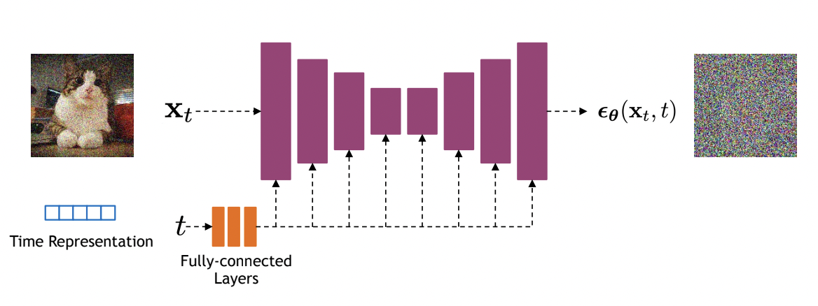

Diffusion models often use U-Net architectures with ResNet blocks and self-attention layers to represent $\epsilon_\theta(\mathbf{x}_t, t)$. Time features (usually sinusoidal positional embeddings or random Fourier features) are fed to the residual blocks using either simple spatial addition or using adaptive group normalization layers. Image source.

To summarize, our training process:

Sample $\mathbf{x}_0 \sim q(\mathbf{x}_0)$
Choose randomly a certain step in diffusion process: $t \sim \mathcal{U}(\lbrace 1,2, \dots T \rbrace)$
Apply noising: $\mathbf{x}_t = \sqrt{\bar\alpha_t}\mathbf{x}_0+\sqrt{1-\bar\alpha_t} \epsilon$ with $\epsilon \sim \mathcal{N}(0, \mathbf{I})$
Take a gradient step on $\nabla_\theta \| \epsilon - \epsilon_\theta(\mathbf{x}_t, t) \|^2$
Repeat until converge

  
import jax.numpy as jnp
from jax import grad, jit, vmap, random

# hyperparameters
img_shape = (256, 256)
T = 1000
key = random.PRNGKey(42)

# linear schedule
betas = jnp.linspace(1e-4, 0.02, T)
alphas = 1 - betas
alpha_bars = jnp.cumprod(alphas)

# initial model weights
dummy = random.uniform(key, shape=img_shape)
params = model.init(key, dummy)

@jit
def loss(params, eps, x_t, t):
    return jnp.sum((eps - model.apply(params, x_t, t)) ** 2)

@jit
def apply_noising(img, a, noise):
    return jnp.sqrt(a) * img + jnp.sqrt(1 - a) * noise
	    
def train_step(x_0):
    # choose random steps
    t = random.randint(key, shape=(x_0.shape[0],), minval=0, maxval=T)
    # add noise
    eps = random.normal(key, shape=x_0.shape)
    x_t = jit(vmap(apply_noising))(x_0, alpha_bars[t], eps)
    # calculate gradients
    grads = jit(grad(loss))(params, eps, x_t)
    # update parameters with gradients and your favourite optimizer
    ...

Inference process consists of the following steps:

Sample $\mathbf{x}_T \sim \mathcal{N}(0, \mathbf{I})$
For $t = T, \dots, 1$

\[\mathbf{x}_{t-1} = \mu_\theta(\mathbf{x}_t, t) + \sigma_t \epsilon,\]

where $\epsilon \sim \mathcal{N}(0, \mathbf{I})$ and

\[\mu_\theta(\mathbf{x}_t, t) = \frac{1}{\sqrt{\bar\alpha_t}}\Big(\mathbf{x}_t - \frac{1-\alpha_t}{\sqrt{1-\bar\alpha_t}}\epsilon_\theta(\mathbf{x}_t, t) \Big).\]

Return $\mathbf{x}_0$

  
def sample_step(params, x_t, t):
    eps = model.apply(params, x_t, t)
    mu_t = x_t - eps * (1 - alphas[t]) / jnp.sqrt(1 - alpha_bars[t])
    mu_t /= jnp.sqrt(alpha_bars[t])
    return mu_t + sigma_t * random.normal(key, shape=x_0.shape)

def sample():
    x_t = random.normal(key, shape=img_shape)
    for t in reversed(range(T)):
        x_t = sample_step(params, x_t, t)
    return x_t

Denoising diffusion implicit models (DDIM)

A critical drawback of these models is that they require many iterations to produce a high quality sample. Reverse diffusion process could have thousands of steps and iterating over all the steps is required to produce a single sample, which is much slower compared to GANs, which only needs one pass through a network. For example, it takes around 20 hours to sample 50k images of size 32 × 32 from a DDPM, but less than a minute to do so from a GAN on a Nvidia 2080 Ti GPU. This becomes more problematic for larger images as sampling 50k images of size 256 × 256 could take nearly 1000 hours on the same GPU.

One simple acceleration method is to reduce diffusion time steps in training. Another one is strided sampling schedule: take sampling update every $[T/S]$ steps to reduce process from $T$ down to $S$ steps. However, both of them lead to immediate worse performance.

In DDPMs, the generative process is defined as the reverse of a particular Markovian diffusion process, meaning that each event $t$ depends only on the state attained in the previous event $t-1$. Song et al. generalized DDPMs via a class of non-Markovian diffusion processes that lead to the same training objective.

We can redefine joint distribution $q(\mathbf{x}_{1 : T} \vert \mathbf{x}_0)$ in a way such that forward process is non-Markovian, while marginals stay the same. Let

\[\begin{aligned} \mathbf{x}_{t-1} \vert \mathbf{x}_t, \mathbf{x}_0 &= \sqrt{\bar\alpha_{t-1}} \mathbf{x}_0 + \sqrt{1 - \bar\alpha_{t-1}} \epsilon_{t-1} & \color{Salmon}{\epsilon_{t-1} \sim \mathcal{N}(0, \mathbf{I})} \\ & = \sqrt{\bar\alpha_{t-1}} \mathbf{x}_0 + \sqrt{1 - \bar\alpha_{t-1} - \sigma_t^2} \epsilon_{t} + \sigma_t \epsilon & \color{Salmon}{\epsilon \sim \mathcal{N}(0, \mathbf{I})} \\ & = \sqrt{\bar\alpha_{t-1}} \mathbf{x}_0 + \sqrt{1 - \bar\alpha_{t-1} - \sigma_t^2} \frac{\mathbf{x}_t - \sqrt{\bar\alpha_t}\mathbf{x}_0}{\sqrt{1-\bar\alpha_t}} + \sigma_t \epsilon \end{aligned}\]

with some deviation process $\sigma_t$. Then we have

\[q_\sigma(\mathbf{x}_{t-1} \vert \mathbf{x}_t, \mathbf{x}_0) = \mathcal{N}(\sqrt{\bar\alpha_{t-1}} \mathbf{x}_0 + \sqrt{1 - \bar\alpha_{t-1} - \sigma_t^2} \frac{\mathbf{x}_t - \sqrt{\bar\alpha_t}\mathbf{x}_0}{\sqrt{1-\bar\alpha_t}}, \sigma^2_t \mathbf{I})\]

and

\[q_\sigma(\mathbf{x}_{t} \vert \mathbf{x}_0) = \mathcal{N}(\sqrt{\bar\alpha_{t}} \mathbf{x}_0, \sqrt{1 - \bar\alpha_{t}} \mathbf{I}).\]

Recall that for Markovian diffusion process we have distribution

\[q(\mathbf{x}_{t-1} \vert \mathbf{x}_t, \mathbf{x}_0) = \mathcal{N}({\color{#5286A5}{\tilde \mu(\mathbf{x}_t, \mathbf{x}_0)}}, {\color{#C19454}{\tilde \beta_t \mathbf{I}}})\]

with

\[{\color{#C19454}{\tilde \beta_t}} = \frac{1-\bar\alpha_{t-1}}{1-\bar\alpha_t} \beta_t.\]

Hence, we can parameterize distribution $q_\sigma(\mathbf{x}_{t-1} \vert \mathbf{x}_t, \mathbf{x}_0)$ with hyperparamer $\eta > 0$, such that

\[\sigma_t^2 = \eta {\color{#C19454}{\tilde \beta_t}}.\]

Different choices of $\eta$ result in different generative processes, all while using the same model $\epsilon_\theta$, so re-training the model is unnecessary. The special case of $\eta = 1$ corresponds to DDPM. Setting $\eta = 0$ makes the sampling process deterministic. Such model is named the denoising diffusion implicit model (DDIM). In general, one can generate samples in autoregressive way by formula

\[\mathbf{x}_{t-1} = \frac{1}{\sqrt{\alpha_t}}(\mathbf{x}_t - \sqrt{1-\bar\alpha_t}\epsilon_\theta(\mathbf{x}_t, t)) + \sqrt{1-\bar\alpha_{t-1} - \sigma_t^2} \epsilon_\theta(\mathbf{x}_t, t) + \sigma_t \epsilon.\]

We can accelerate inference process by only sampling a subset of $S$ diffusion steps $\lbrace \tau_1, \dots, \tau_S \rbrace$.

Accelerated generation with DDIM and $\tau = [1, 3]$.

  
def sample_step(params, x_t, t):
    eps = model.apply(params, x_t, t)
    x_0_scaled = (x_t - eps * jnp.sqrt(1 - alpha_bars[t])) / jnp.sqrt(alphas[t])
    mu_t = x_0_scaled + jnp.sqrt(1 - alpha_bars[t-1] - sigma_t ** 2)
    return mu_t + sigma_t * random.normal(key, shape=x_0.shape)
    
def sample(taus):
    x_t = random.normal(key, shape=img_shape)
    for t in reversed(taus):
        x_t = sample_step(params, x_t, t)
    return x_t

Score based generative modelling

Diffusion model is an example of discrete Markov chain. We can extend it to continuous stochastic process. Let’s define Wiener process (Brownian motion) $\mathbf{w}_t$ - a random process, such that it starts with $0$, its samples are continuous paths and all of its increments are independent and normally distributed, i.e.

\[\frac{\mathbf{w}(t) - \mathbf{w}(s)}{\sqrt{t - s}} \sim \mathcal{N}(0, \mathbf{I}), \quad t > s.\]

Let also

\[\mathbf{x}\big(\frac{t}{T}\big) := \mathbf{x}_t \ \text{ and } \ \beta\big(\frac{t}{T}\big) := \beta_t \cdot T,\]

then

\[\mathbf{x}\big(\frac{t + 1}{T}\big) = \sqrt{1-\frac{\beta(t/T)}{T}} \mathbf{x}(t/T) + \sqrt{\beta(t/T)} \Big( \mathbf{w}\big(\frac{t+1}{T}\big)-\mathbf{w}\big(\frac{t}{T}\big) \Big).\]

Rewriting equation above with $t:=\frac{t}{T}$ and $\Delta t := \frac{1}{T}$, we get

\[\begin{aligned} \mathbf{x}(t+\Delta t) &= \sqrt{1-\beta(t)\Delta t} \mathbf{x}(t) + \sqrt{\beta(t)} (\mathbf{w}(t + \Delta t)-\mathbf{w}(t)) \\ & \approx \Big(1 - \frac{\beta(t) \Delta t}{2} \Big) \mathbf{x}(t) + \sqrt{\beta(t)}(\mathbf{w}(t + \Delta t)-\mathbf{w}(t)). & \color{Salmon}{\leftarrow \text{Taylor expansion}} \end{aligned}\]

With $\Delta t \rightarrow 0$ this converges to stochastic differential equation (SDE):

\[d\mathbf{x} = -\frac{1}{2}\beta(t)\mathbf{x}dt + \sqrt{\beta(t)} d\mathbf{w}.\]

The equation of type

\[d\mathbf{x} = f(\mathbf{x}, t)dt + g(t)d\mathbf{w}\]

has a unique strong solution as long as the coefficients are globally Lipschitz in both state and time (Øksendal (2003)). We hereafter denote by $q_t(\mathbf{x})$ probability density of $\mathbf{x}(t)$.

By starting from samples of $\mathbf{x}_T \sim q_T(\mathbf{x})$ and reversing the process, we can obtain samples $\mathbf{x}_0 \sim q_0(\mathbf{x})$. It was proved by Anderson (1982) that the reverse of a diffusion process is also a diffusion process, running backwards in time and given by the reverse-time SDE:

\[\begin{aligned} d\mathbf{x} = [f(\mathbf{x}, t) - g(t)^2 &\underbrace{\nabla_{\mathbf{x}} \log q_t(\mathbf{x})}]dt + g(t) d\bar{\mathbf{w}}, &\\ &\color{Salmon}{\text{Score Function}} \\ \end{aligned}\]

where $\bar{\mathbf{w}}$ is a standard Wiener process when time flows backwards from $T$ to $0$. In our case with

\[f(\mathbf{x},t) = -\frac{1}{2}\beta(t)\mathbf{x}(t) \ \text{ and } \ g(t) = \sqrt{\beta(t)}\]

we have reverse diffusion process

\[d\mathbf{x} = \big[-\frac{1}{2}\beta(t)\mathbf{x} - \beta(t) \nabla_{\mathbf{x}} \log q_t(\mathbf{x})\big] dt + \sqrt{\beta(t)}d\bar{\mathbf{w}}.\]

Once the score of each marginal distribution is known for all $t$, we can map data to a noise (prior) distribution with a forward SDE, and reverse this SDE for to sample from $q_0$.

Forward and reverse generative diffusion SDEs.

In order to estimate $\nabla_{\mathbf{x}} \log q_t(\mathbf{x})$ we can train a time-dependent score-based model $\mathbf{s}_\theta(\mathbf{x}, t)$, such that

\[\mathbf{s}_\theta(\mathbf{x}, t) \approx \nabla_{\mathbf{x}} \log q_t(\mathbf{x}).\]

The marginal diffused density $q_t(\mathbf{x}(t))$ is not tractable, however,

\[q_t(\mathbf{x}(t) \vert \mathbf{x}(0)) \sim \mathcal{N}(\sqrt{\bar{\alpha}(t)} \mathbf{x}(0), (1 - \bar{\alpha}(t)) \mathbf{I})\]

with $\bar{\alpha}(t) = e^{\int_0^t \beta(s) ds}$. Therefore we can minimize

\[\mathcal{L} = \mathbb{E}_{t \sim \mathcal{U}(0, t)} \mathbb{E}_{\mathbf{x}(0) \sim q_0(\mathbf{x})} \mathbb{E}_{\mathbf{x}(t) \sim q_t(\mathbf{x}(t) \vert \mathbf{x}(0))}[ \| \mathbf{s}_\theta(\mathbf{x}(t), t) - \nabla_{\mathbf{x}(t)} \log q_t(\mathbf{x}(t) \vert \mathbf{x}(0)) \|^2 ].\]

Connection to diffusion model

Given a Gaussian distribution

\[\mathbf{x}(t) = \sqrt{\bar{\alpha}(t)} \mathbf{x}(0) + \sqrt{1 - \bar{\alpha}(t)} \epsilon, \quad \epsilon \sim \mathcal{N}(0, \mathbf{I}),\]

we can write the derivative of the logarithm of its density function as

\[\begin{aligned} \nabla_{\mathbf{x}(t)} \log q_t(\mathbf{x}(t) \vert \mathbf{x}(0)) &= -\nabla_{\mathbf{x}(t)} \frac{(\mathbf{x}(t) - \sqrt{\bar{\alpha}(t)} \mathbf{x}(0))^2}{2 (1 - \bar{\alpha}(t))} \\ &= -\frac{\mathbf{x}(t) - \sqrt{\bar{\alpha}(t)} \mathbf{x}(0)}{1 - \bar{\alpha}(t)} \\ &= \frac{\epsilon}{\sqrt{1 - \bar{\alpha}(t)}}. \end{aligned}\]

Also,

\[\mathbf{s}_\theta(\mathbf{x}, t) = -\frac{\epsilon_\theta(\mathbf{x}, t)}{\sqrt{1 - \bar{\alpha}(t)}}.\]

Guided diffusion

Once the model $\epsilon_\theta(\mathbf{x}_t, t)$ is trained, we can use it to run the isotropic Gaussian distribution $\mathbf{x}_T$ back to $\mathbf{x}_0$ and generate limitless image variations. But how can we guide the class-conditional model to generate specific images by feeding additional information about class $y$ during the training process?

Classifier guidance

If we have a differentiable discriminative model $f_\phi(y \vert \mathbf{x}_t)$, trained to classify noisy images $\mathbf{x}_t$, we can use its gradients to guide the diffusion sampling process toward the conditioning information $y$ by altering the noise prediction.

We can write the score function for the joint distribution $q(\mathbf{x}, y)$ as following,

\[\begin{aligned} \nabla_{\mathbf{x}_t} \log q(\mathbf{x}_t, y) &= \nabla_{\mathbf{x}_t} \log q(\mathbf{x}_t) + \nabla_{\mathbf{x}_t} \log q(y \vert \mathbf{x}_t) \\ & \approx -\frac{\epsilon_\theta(\mathbf{x}_t, t)}{\sqrt{1 - \bar{\alpha}_t}} + \nabla_{\mathbf{x}_t} \log f_\phi (y \vert \mathbf{x}_t) \\ &= -\frac{1}{\sqrt{1 - \bar{\alpha}_t}}\big(\epsilon_\theta(\mathbf{x}_t, t) - \sqrt{1 - \bar{\alpha}_t}\nabla_{\mathbf{x}_t} \log f_\phi (y \vert \mathbf{x}_t)\big). \end{aligned}\]

At each step of denoising, the classifier checks whether the image is denoised in the right direction and contributes its own gradient of loss function into the overall loss of diffusion model. To control the strength of the classifier guidance, we can add a weight $\omega$, called the guidance scale, and here is our new classifier-guided model:

\[\tilde{\epsilon}_\theta(\mathbf{x}_t, t) = \epsilon_\theta(\mathbf{x}_t, t) - \omega \sqrt{1 - \bar{\alpha}_t} \nabla_{\mathbf{x}_t} \log f_\phi (y \vert \mathbf{x}_t).\]

We can then use the exact same sampling procedure, but with the modified noise predictions $\tilde{\epsilon}_\theta$. This results in approximate sampling from distribution:

\[\tilde{q}(\mathbf{x}_t \vert y) \propto q(\mathbf{x}_t) \cdot q(y \vert \mathbf{x}_t)^\omega.\]

Basically, we are raising the conditional part of the distribution to a power, which corresponds to tuning the inverse temperature of that distribution. With large $\omega$ we focus onto distribution modes and produce higher fidelity (but less diverse) samples.

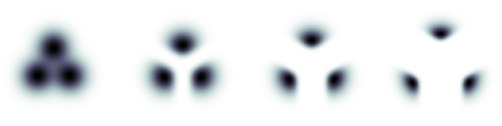Guidance on a toy 2D example of three classes, in which the conditional distribution for each class is an isotropic Gaussian, each mixture component representing data conditioned on a class. The leftmost plot is the non-guided marginal density. Left to right are densities of mixtures of normalized guided conditionals with increasing guidance strength. Image source

A downside of classifier guidance is that it requires an additional classifier model and thus complicates the training pipeline. One can’t plug in a standard pre-trained classifier, because this model has to be trained on noisy data $\mathbf{x}_t$. And even having a classifier, which is robust to noise, classifier guidance is inherently limited in its effectiveness. Most of the information in the input $\mathbf{x}_t$ is not relevant to predicting $y$, and as a result, taking the gradient of the classifier w.r.t. its input can yield arbitrary (and even adversarial) directions in input space.

Classifier-free guidance

Ho & Salimans proposed an alternative method, a classifier-free guidance, which doesn’t require training a separate classifier. Instead, one trains a conditional diffusion model, parameterized by $\epsilon_\theta(\mathbf{x}_t, t \vert y)$ with conditioning dropout: 10-20% of the time, the conditioning information $y$ is removed. In practice, it is replaced with a special input value $y=\emptyset$ representing the absence of conditioning information. This way model knows how to generate images unconditionally as well, i.e.

\[\epsilon_\theta(\mathbf{x}_t, t) = \epsilon_\theta(\mathbf{x}_t, t \vert \emptyset).\]

How could we use it for sampling? By Bayes rule we have

\[\begin{aligned} q(y \vert \mathbf{x}_t) &= \frac{q(\mathbf{x}_t \vert y) q(y)}{q(\mathbf{x}_t)} \\ \Longrightarrow \nabla_{\mathbf{x}_t} \log q(y \vert \mathbf{x}_t) &= \nabla_{\mathbf{x}_t} \log q(\mathbf{x}_t \vert y) - \nabla_{\mathbf{x}_t} \log q(\mathbf{x}_t) \\ & \approx -\frac{\epsilon_\theta(\mathbf{x}_t, t \vert y) - \epsilon_\theta(\mathbf{x}_t, t)}{\sqrt{1 -\bar{\alpha}_t}}. \end{aligned}\]

Substituting this into the formula for classifier guidance, we get

\[\begin{aligned} \tilde{\epsilon}_\theta(\mathbf{x}_t, t \vert y) &= \epsilon_\theta(\mathbf{x}_t, t) - \omega \sqrt{1 - \bar{\alpha}_t} \nabla_{\mathbf{x}_t} \log q(y \vert \mathbf{x}_t) \\ &= (1-\omega) \epsilon_\theta(\mathbf{x}_t, t) + \omega\epsilon_\theta(\mathbf{x}_t, t \vert y). \end{aligned}\]

The classifier-free guided model is a linear interpolation between models with and without labels: for $\omega=0$ we get unconditional model, and for $\omega=1$ we get the standard conditional model. However, as experiments have shown in Dhariwal & Nichol paper, guidance works even better with $\omega > 1$.

Note on notation: authors of original paper applied classifier guidance to already conditional diffusion model $\epsilon(\mathbf{x}_t, t \vert y)$:

\[\begin{aligned} \tilde{\epsilon}_\theta(\mathbf{x}_t, t \vert y) &= \epsilon_\theta(\mathbf{x}_t, t \vert y) - \omega \sqrt{1 - \bar{\alpha}_t} \nabla_{\mathbf{x}_t} \log q(y \vert \mathbf{x}_t) \\ &= (\omega + 1) \epsilon_\theta(\mathbf{x}_t, t \vert y) - \omega\epsilon_\theta(\mathbf{x}_t, t). \end{aligned}\]

This is the same as applying guidance to unconditional model with $\omega + 1$ scale, because

\[\tilde{q}(\mathbf{x}_t \vert y) \propto q(\mathbf{x}_t \vert y) \cdot q(y \vert \mathbf{x}_t)^\omega \propto q(\mathbf{x}_t) \cdot q(y \vert \mathbf{x}_t)^{\omega+1}.\]

CLIP guidance

With CLIP guidance the classifier is replaced with a CLIP model (abbreviation for Contrastive Language-Image Pre-training). CLIP was originally a separate auxiliary model to rank the results from generative model, called DALL·E. DALL·E was the first public system capable of creating images based on a textual description from OpenAI, however it was not a diffusion model and is therefore out of the scope for this post. DALL·E’s name is a portmanteau of the names of animated robot Pixar character WALL-E and the Spanish surrealist artist Salvador Dalí.

The idea behind CLIP is fairly simple:

Take two encoders, one for a text snippet and another one for an image
Collect a sufficiently large dataset of image-text pairs (e.g. 400 million scraped from the Internet in the paper)
Train the model in a contrastive fashion: it must produce high similarity score for an image and a text from the same pair and a low similarity score for mismatched image and text.

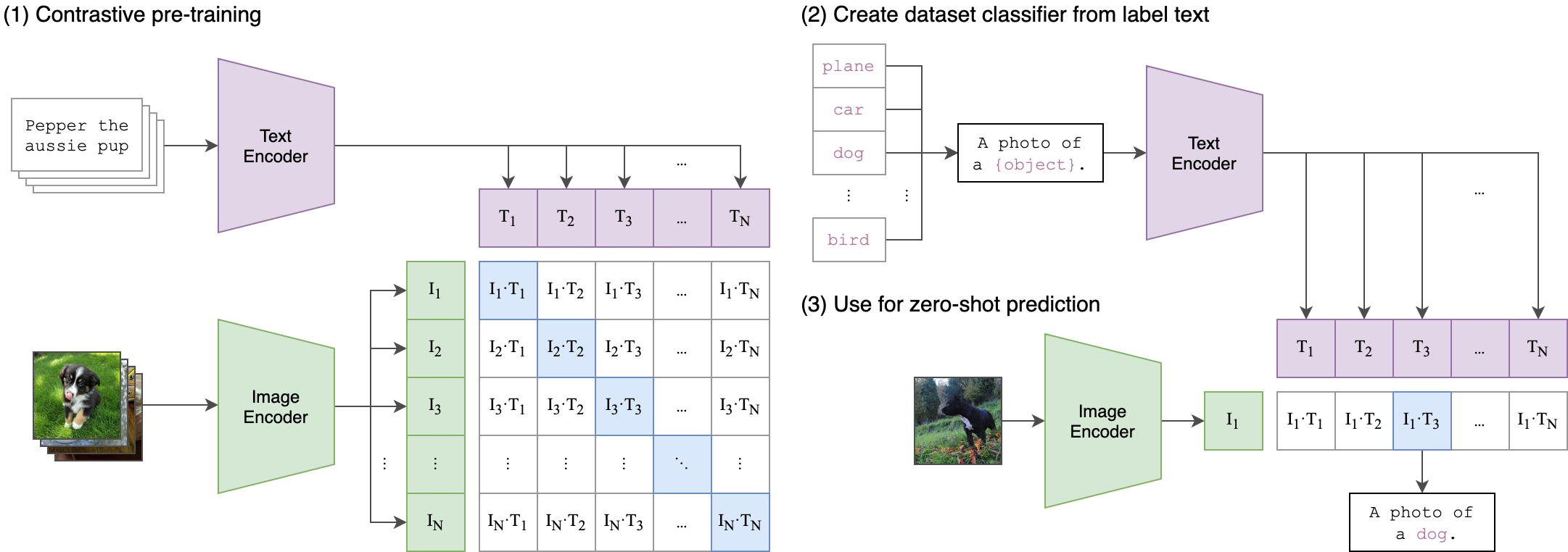CLIP approach: jointly train an image encoder and a text encoder to predict the correct pairings of a batch of (image, text) training examples. At test time the learned text encoder synthesizes a zero-shot linear classifier by embedding the names or descriptions of the target dataset’s classes. The classes can be adjustable without retraining a model.

  
# image_encoder - ResNet or Vision Transformer
# text_encoder - CBOW or Text Transformer
# I[n, h, w, c] - minibatch of aligned images
# T[n, l] - minibatch of aligned texts
# W_i[d_i, d_e] - learned proj of image to embed
# W_t[d_t, d_e] - learned proj of text to embed
# tau - learned temperature parameter

# extract feature representations of each modality
I_f = image_encoder(I) #[n, d_i]
T_f = text_encoder(T) #[n, d_t]

# joint multimodal embedding [n, d_e]
I_e = l2_normalize(jnp.dot(I_f, W_i), axis=1)
T_e = l2_normalize(jnp.dot(T_f, W_t), axis=1)

# scaled pairwise cosine similarities [n, n]
logits = jnp.dot(I_e, T_e.T) * jnp.exp(tau)

# symmetric loss function
labels = jnp.arange(n)
loss_i = cross_entropy_loss(logits, labels, axis=0)
loss_t = cross_entropy_loss(logits, labels, axis=1)
loss = (loss_i + loss_t) / 2

Let $f(\mathbf{x})$ and $g(y)$ be image and text encoders respectively. Then CLIP loss for $(i, j)$ pair is

\[\begin{aligned} \mathcal{L}_{\operatorname{CLIP}}(i, j) &= \frac{1}{2} \bigg(-\log \frac{\exp(f(\mathbf{x}_i) \cdot g(y_j) / \tau)}{\sum_k \exp(f(\mathbf{x}_i) \cdot g(y_k) / \tau)}-\log \frac{\exp(f(\mathbf{x}_i) \cdot g(y_j) / \tau)}{\sum_k \exp(f(\mathbf{x}_k) \cdot g(y_j) / \tau)} \bigg). \end{aligned}\]

Ideally, we get

\[f(\mathbf{x}) \cdot g(y) \approx \frac{q(\mathbf{x}, y)}{q(\mathbf{x}) q(y)} = \frac{q(y \vert \mathbf{x})}{ q(y)},\]

which can be used to steer generative models instead of pretrained classifier:

\[\begin{aligned} \nabla_{\mathbf{x}_t} \log q(\mathbf{x}_t, y) &= \nabla_{\mathbf{x}_t} \log q(\mathbf{x}_t) + \nabla_{\mathbf{x}_t} \log q(y \vert \mathbf{x}_t) \\&= \nabla_{\mathbf{x}_t} \log q(\mathbf{x}_t) + \nabla_{\mathbf{x}_t} (\log q(y \vert \mathbf{x}_t) -\log q(y)) \\ & \approx -\frac{\epsilon_\theta(\mathbf{x}_t, t)}{\sqrt{1 - \bar{\alpha}_t}} + \nabla_{\mathbf{x}_t} \log (f(\mathbf{x}_t) \cdot g(y)). \end{aligned}\]

Similar to classifier guidance, CLIP must be trained on noised images $\mathbf{x}_t$ to obtain the correct gradient in the reverse process.

GLIDE

GLIDE, which stands for Guided Language to Image Diffusion for Generation and Editing, is a model by OpenAI that has beaten DALL·E, arguably presented the most novel and interesting ideas and yet received comparatively little publicity.

Motivated by the ability of guided diffusion models to generate photorealistic samples and the ability of text-to-image models to handle free-form prompts, authors of the paper applied guided diffusion to the problem of text-conditional image synthesis. They also compared two techniques for guiding diffusion models towards text prompts: CLIP guidance and classifier-free guidance. Using human and automated evaluations, they found that classifier-free guidance yields higher-quality images.

An architecture of GLIDE consists of three major blocks:

U-Net based text-conditional diffusion model at 64 × 64 resolution (2.3B parameters)
Transformer based text encoder to condition on natural language descriptions (1.2B parameters)
Another text-conditional upsampling diffusion model to increase the resolution to 256 × 256 (1.5B parameters)

The U-Net model as usual stacks residual layers with downsampling convolutions, followed by a stack of residual layers with upsampling convolutions, with skip connections connecting the layers with the same spatial size. It also consists of attention layers which are crucial for simultaneous text processing.

The text encoder was built from 24 residual blocks of width 2048. The input is a sequence of $K$ tokens. The output of the transformer is used in two ways:

the final token embedding token is used in place of a class embedding $y$,
the final layer of token embeddings is added to every attention layer of the model.

Model has fewer parameters than DALL·E (5B vs 12B) and was trained on the same dataset, however was favored over it by human evaluators and has beaten it by FID score. However, as the authors mentioned, unoptimized GLIDE takes 15 seconds to sample one image on a single A100 GPU. This is much slower than sampling for related GAN methods, which produce images in a single forward pass and are thus more favorable for use in real-time applications.

DALL·E 2 (unCLIP)

In April 2022, OpenAI released a new model, called DALL·E 2 (or unCLIP in the paper), which is a clever combination of CLIP and GLIDE. The CLIP model is trained separately on a data of image-text pairs $(\mathbf{x}, y)$. Let

\[\mathbf{z}_i = \operatorname{CLIP}(\mathbf{x}) \quad \text{and} \quad \mathbf{z}_t = \operatorname{CLIP}(y)\]

be CLIP image and text embeddings respectively. In the paper Vision Transformer was used as image encoder and Transformer with a causal attention mask as text encoder. Then CLIP is frozen and the unCLIP learns two models in parallel:

a special prior model $q(\mathbf{z}_i \vert y)$ outputs CLIP image embedding given the text $y$,
a diffusion decoder (modified GLIDE) $q(\mathbf{x} \vert \mathbf{z}_i, [y])$ generates the image $\mathbf{x}$ given CLIP image embedding $\mathbf{z}_i$ and optionally the original text $y$.

Stacking these two components yields a generative model of images $\mathbf{x}$ given captions $y$:

\[q(\mathbf{x} \vert y) = q(\mathbf{x}, \mathbf{z}_i \vert y) = q(\mathbf{x} \vert \mathbf{z}_i, y) \cdot q(\mathbf{z}_i \vert y).\]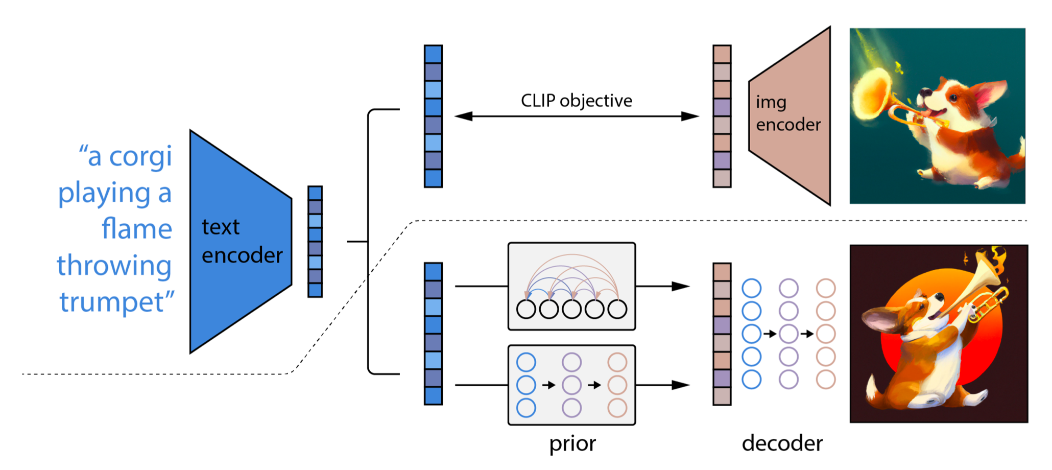

unCLIP architecture. Below the dotted line the text-to-image process is depicted. Given a text $y$ the CLIP text encoder generates a text embedding $\mathbf{z}_t$. Then a diffusion or autoregressive prior model processes this CLIP text embedding to construct an image embedding $\mathbf{z}_i$. Then a diffusion decoder generates images conditioned on CLIP image embeddings (and text). The decoder essentially inverts image embeddings back into images

The authors tested two model classes for the prior:

Autoregressive prior quantizes image embedding to a sequence of discrete codes and predict them autoregressively.
Diffusion prior models the continuous image embedding by diffusion models conditioned on $y$.

Diffusion prior outperforms the autoregressive prior for comparable model size and reduced training compute. The diffusion prior also performs better than the autoregressive prior in pairwise comparisons against GLIDE.

As opposed to the way of training proposed by Ho et al., predicting the unnoised image embedding directly instead of predicting the noise was a better fit. Meaning, that instead of

\[L_t = \mathbb{E}_{\mathbf{x}_0, \epsilon} \big[ \|\epsilon - \epsilon_\theta(\mathbf{x}_t, t \vert y) \|^2 \big]\]

the unCLIP diffusion prior loss is

\[L_t = \mathbb{E}_{\mathbf{x}_0, \epsilon} \big[ \| \mathbf{z}_i - f_\theta(\mathbf{z}_i^{(t)}, t \vert y) \|^2 \big],\]

where $f_\theta$ stands for the prior model and $\mathbf{z}_i^{(t)}$ is the noised image embedding.

The bipartite latent representation enables several text-guided image manipulation tasks. For example, one can fix CLIP image embeddings $\mathbf{z}_i$ and run decoder with different decoder latents $\mathbf{x}_T$.

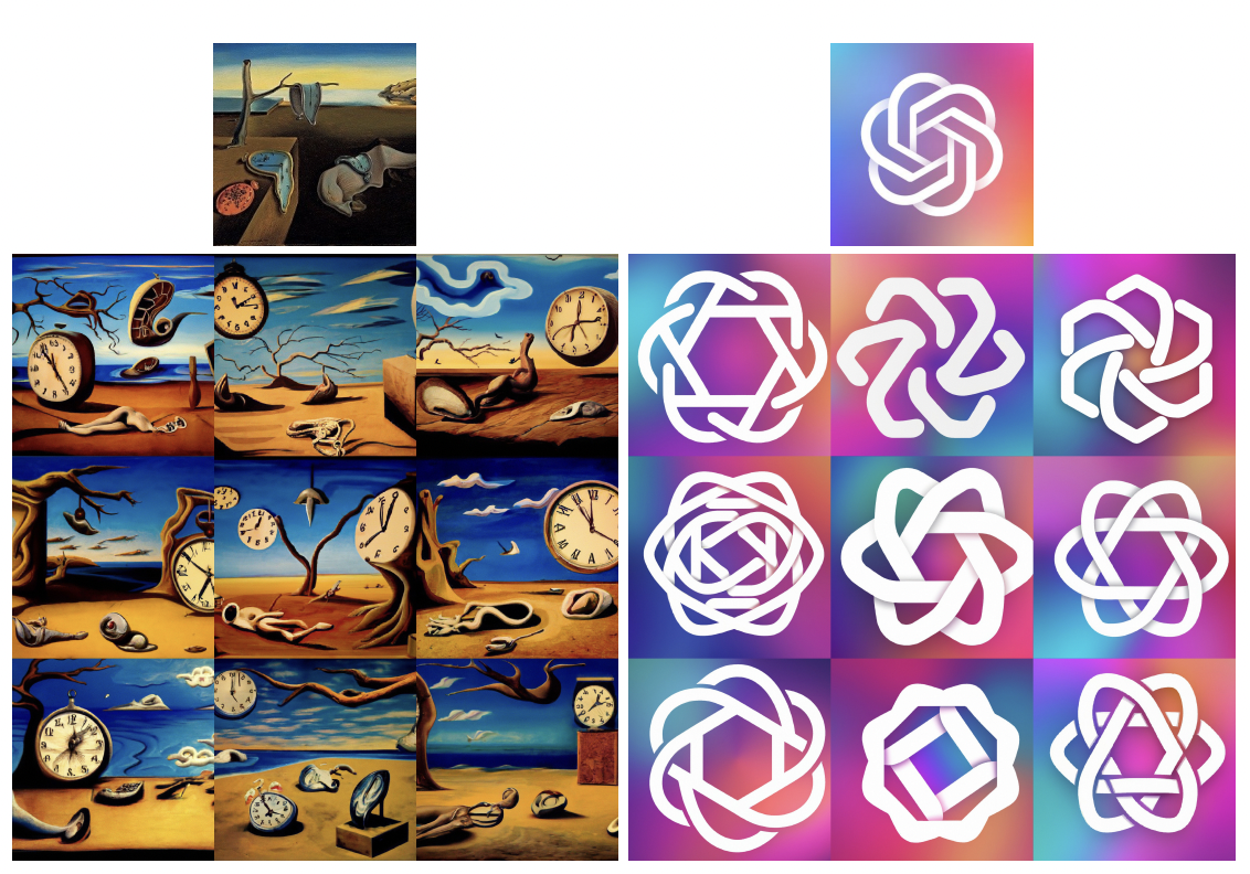Variations of an input image by encoding with CLIP and then decoding with a diffusion model. The variations preserve both semantic information like presence of a clock in the painting and the overlapping strokes in the logo, as well as stylistic elements like the surrealism in the painting and the color gradients in the logo, while varying the non-essential details.

Or one can change $\mathbf{z}_i$ towards the difference of the text CLIP embeddings $\mathbf{z}_t$ of two prompts.

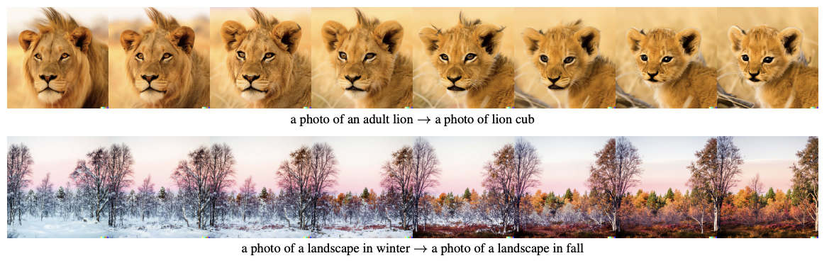Text diffs applied to images by interpolating between their CLIP image embeddings and a normalised difference of the CLIP text embeddings produced from the two descriptions. Decoder latent $\mathbf{x}_T$ is kept as a constant.

Imagen

Two months after the publication of DALL·E 2 Google Brain team presented Imagen. It uses a pre-trained T5-XXL language model instead of CLIP to encode text for image generation. The idea is that this model has vastly more context regarding language processing than a model trained only on the image captions, and so is able to produce more valuable embeddings without the need to additionally fine-tune it. Authors of the paper noted, that scaling text encoder is extremely efficient and more important than scaling diffusion model size.

Next, the resolution is increased via super-resolution diffusion models. There is another key observation from authors: noise conditioning augmentation weakens information from low-resolution models, thus it is beneficial to use text conditioning as extra information input.

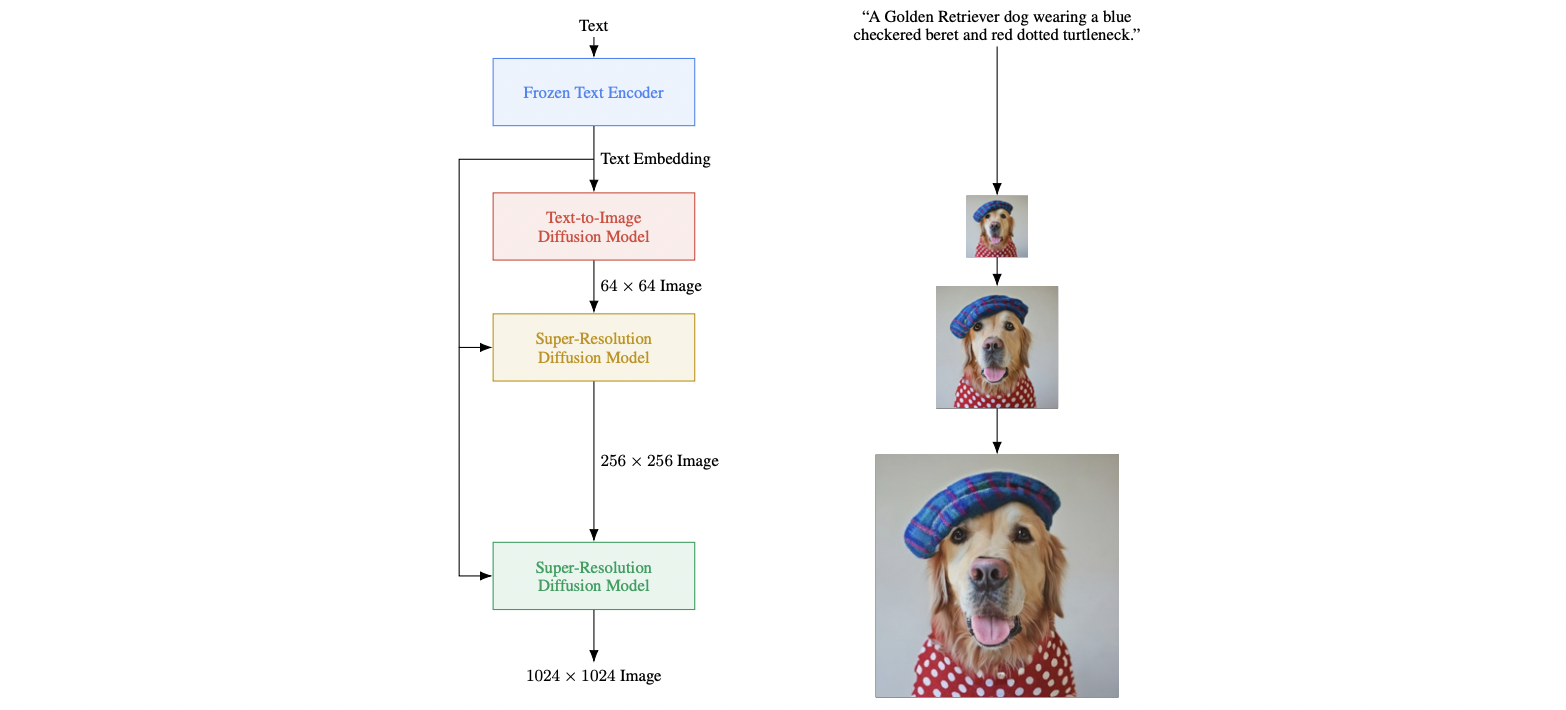Visualization of Imagen. Imagen uses a frozen text encoder to encode the input text into text embeddings. A conditional diffusion model maps the text embedding into a 64 × 64 image. Imagen further utilizes text-conditional super-resolution diffusion models to upsample the image, first 64 × 64 → 256 × 256, and then 256 × 256 → 1024 × 1024.

Noise conditioning augmentation

The solution can be viewed as a sequence of diffusion models, which was called cascaded diffusion models in Ho et al. (2021). Noise conditioning augmentation between these models is crucial to the final image quality, which is to apply strong data augmentation to the low-resolution image $\mathbf{z}$ of each super-resolution model $p_\theta(\mathbf{x} \vert \mathbf{z})$. In simple terms, it is equivalent to applying various data augmentation techniques, such as a Gaussian noise/blur, to a low-resolution image before it is fed into the super-resolution models.

  
def train_step_base(z_0):
    # diffusion forward process
    s = random.randint(key, shape=(z.shape[0],), minval=0, maxval=T)
    eps = random.normal(key, shape=z.shape)
    z_s = jit(vmap(apply_noising))(z, alpha_bars[s], eps)
    # optimize loss(z_0, model(z_s, s))
    ...
    
def train_step_sr(z_0, x_0):
    # add gaussian conditioning augmentation to the low-resolution image
    s = random.randint(key, shape=(z_0.shape[0],), minval=0, maxval=T)
    eps_z = random.normal(key, shape=z_0.shape)
    z_0 = jit(vmap(apply_noising))(z_0, alpha_bars[s], eps_z)    
    # diffusion forward process
    t = random.randint(key, shape=(x_0.shape[0],), minval=0, maxval=T)
    eps_x = random.normal(key, shape=x_0.shape)
    x_t = jit(vmap(apply_noising))(x_0, alpha_bars[t], eps_x)
    # optimize loss(x_0, model(x_t, z_0, t, s))
    ...

In addition, there are also two similar forms of conditioning augmentation that require small modification to the training process:

Truncated conditioning augmentation stops the diffusion process early at step $t > 0$ for low resolution.
Non-truncated conditioning augmentation runs the full low resolution reverse process until step $0$ but then corrupt it by $\mathbf{z}_t’ \sim q(\mathbf{z}_t \vert \mathbf{z}_0)$ and then feeds the corrupted $\mathbf{z}_t’$ into the super-resolution model.

  
def sample_step(params, x_t, t, condition=None):
    eps = model.apply(params, x_t, t, condition)
    mu_t = x_t - eps * (1 - alphas[t]) / jnp.sqrt(1 - alpha_bars[t])
    mu_t /= jnp.sqrt(alpha_bars[t])
    return mu_t + sigma_t * random.normal(key, shape=x_0.shape)

def sample_base():
    z_t = random.normal(key, shape=img_shape)
    for t in reversed(range(s, T)):
        z_t = sample_step(params, z_t, t)
    if not_using_truncated:
        for t in reversed(range(s)):
            z_t = sample_step(params, z_t, t)
        eps_z = random.normal(key, shape=z_t.shape)
        z_t = apply_noising(z_t, alpha_bars[s], eps_z)
    return z_t

def sample_sr():
    # sample augmented low-resolution image
    z_0 = sample_base()
    # sample high-resolution image
    x_t = random.normal(key, shape=img_shape)
    for t in reversed(range(T)):
        x_t = sample_step(params, x_t, t, z_t)
    return x_t

Dynamic thresholding

Another major key feature of Imagen is a so-called dynamic thresholding. Authors of the model found out that larger classifier-free guidance scale $\omega$ leads to better text alignment, but worse image fidelity producing highly saturated and unnatural images. They hypothesised that large $\omega$ increases train-test mismatch and generated images are saturated due to the very large gradient updates during sampling.

At each sampling step $t$, the prediction $\mathbf{x}_t$ must be within the same bounds as training data, i.e. within $[−1, 1]$, but authors of Imagen found empirically that high guidance weights cause predictions to exceed these bounds. To counter this problem, they proposed to adjust the pixel values of samples at each sampling step to be within this range. Basically, two approaches could be applied:

Static thresholding: clip $\mathbf{x}_t$ to $[-1, 1]$.
Dynamic thresholding: at each sampling step $t$, compute $s$ as a certain $p$-percentile absolute pixel value; if $s > 1$ clip the prediction to $[-s, s]$ and divide by $s$.

  
def sample():
    x_t = random.normal(key, shape=img_shape)
    for t in reversed(range(T)):
        x_t = sample_step(params, x_t, t)
        if using_static:
            x_t = jnp.clip(x_t, -1.0, 1.0)
        else:
            s = jnp.percentile(jnp.abs(x_t), p, axis=tuple(range(1, x_t.ndim)))
            s = jnp.max(s, 1.0)
            x_t = jnp.clip(x_t, -s, s) / s
    return x_t

Latent-space diffusion model / Stable diffusion

Rombach & Blattmann, et al. 2022 presented latent diffusion models (LDM), which operate in the latent space of pretrained variational autoencoders instead of pixel space, making training cost lower and inference speed faster.

The diffusion and denoising processes happen on a 2D latent vector $\mathbf{z}$, which is an image $\mathbf{x}$, compressed by encoder. Then an decoder reconstructs the images from the latent vector. The paper explored two types of regularization in autoencoder training to avoid arbitrarily high-variance in the latent spaces:

KL-regularization: a small KL penalty towards a standard normal distribution over the learned latent, similar to VAE.
VQ-regularization: Uses a vector quantization layer within the decoder, like VQVAE but the quantization layer is absorbed by the decoder.

The denoising model is a time-conditioned U-Net. Authors also introduced cross-attention layers into the model architecture to handle flexible conditioning information. Each type of conditioning information is paired with a domain-specific encoder $\tau_\theta$ to project the conditioning input $y$ to an intermediate representation, which is then mapped to the intermediate layers of the UNet via a cross-attention layer implementing

\[\operatorname{Attention}(\mathbf{Q}, \mathbf{K}, \mathbf{V}) = \operatorname{softmax} \Big( \frac{\mathbf{QK}^T}{\sqrt{d}} \Big) \cdot \mathbf{V},\]

where

\[\mathbf{Q} = \mathbf{W}_Q^{(i)} \cdot \varphi_i(\mathbf{z}_t), \ \mathbf{K} =\mathbf{W}_K^{(i)} \cdot \tau_\theta(y), \ \mathbf{V} =\mathbf{W}_V^{(i)} \cdot \tau_\theta(y).\]

Here $\varphi_i$ denotes a (flattened) intermediate representation of the UNet implementing $\epsilon_\theta$.

The architecture of latent diffusion model.

In 2022 in collaboration with Stability AI and Runway a text-to-image LDM called Stable Diffusion was released. Stable Diffusion was trained on 256x256 (then finetuned on 512x512) images from a subset of the LAION-Aesthetics V2 dataset, using 256 Nvidia A100 GPUs on Amazon Web Service for a total of 150,000 GPU-hours, at a cost of $600,000.

Similar to Google’s Imagen, this model uses a frozen CLIP ViT-L/14 text encoder to condition the model on text prompts. With its 860M UNet and 123M text encoder, the model is relatively lightweight and runs on a GPU with at least 10GB VRAM.

Stable diffusion samples.

Unlike previous models, Stable Diffusion makes its source code available, along with pre-trained weights.

Conclusion

Diffusion models have shown amazing capabilities as generative models. They are both analytically tractable and flexible: they can be analytically evaluated and cheaply fit arbitrary structures in data. Besides text-conditioned image generation there a lot of interesting characteristics of the models which were not covered in this post, such as image in-/outpainting, style transfer and image editing.

On the other hand, there is a shortcoming embedded into the diffusion process structure: the sampling relies on a long Markov chain of diffusion steps and it is still slower than GAN. Latent diffusion models have shown that performance gains can be achieved by learning semantically meaningful latent space with complex compressing encoders.

Generative AI, Diffusion Models

This post is licensed under CC BY 4.0 by the author.