Exploring Parallel Strategies with Jax
Training large language models either like GPT, LlaMa or Mixtral requires immense computational resources. With model sizes ballooning into the billions or sometimes even trillions of parameters, specialized parallelization techniques are essential to make training feasible. In this post, we’ll explore implementing some of these scaling strategies in Jax - a Python framework designed for high-performance numerical computing with support for accelerators like GPU and TPU.
Tensors sharding
Jax is a great fit for implementing parallel LLM training thanks to its high-level APIs for composing parallel functions and its seamless acceleration on GPU/TPU hardware. We’ll walk through code examples for data, tensor, pipeline and expert parallelisms in Jax while training a “toy” FFN model for demonstration. The insights from this exercise will help us understand how state-of-the-art systems actually parallelize and distribute LLM training in practice.
Device placement
First, let’s discover how to run particular operations on a device of your choice. Don’t worry if you don’t have multiple GPUs, an arbitrary number of devices can be emulated even with single CPU by setting --xla_force_host_platform_device_count flag:
1
2
3
4
5
6
import os
import jax
import jax.numpy as jnp

# Use 8 CPU devices
os.environ["XLA_FLAGS"] = '--xla_force_host_platform_device_count=8'
With this little trick jax.devices() now shows us eight “different” devices:
1
2
[CpuDevice(id=0), CpuDevice(id=1), CpuDevice(id=2), CpuDevice(id=3),
 CpuDevice(id=4), CpuDevice(id=5), CpuDevice(id=6), CpuDevice(id=7)]
Let’s create a small empty tensor x and observe its physical location:
1
2
3
batch_size, embed_dim = 16, 8
x = jnp.zeros((batch_size, embed_dim))
print(x.devices()) # will output default device, e.g. {CpuDevice(id=0)}
To put tensor x on specific device one can simply use device_put function:
1
jax.device_put(x, jax.devices()[1]).device() # {CpuDevice(id=1)}
What if we want to place different parts of our tensor on different devices? There is a technique called tensor sharding: we split x by multiple sub-tensors and place each on its own device. But before we do that, we need to create a sharding object, which is basically a device placement configuration:
1
2
3
from jax.sharding import PositionalSharding

sharding = PositionalSharding(jax.devices())
We can split our tensor x in multiple ways. For example, we can split it column-wise along embedding dimension:
1
2
G = jax.local_device_count()
sharded_x = jax.device_put(x, sharding.reshape(1, G))
If we print sharded_x.devices() it will give us a list of all devices, which is not very informative since it tells us nothing about our tensor sharding. Luckily, we have visualize_array_sharding function from jax.debug which gives us a pretty visual idea on how x is sharded:
1
2
3
4
5
6
7
from jax.debug import visualize_array_sharding
import matplotlib as mpl

def visualize(tensor, color_map="Set3"):
    visualize_array_sharding(tensor, color_map=mpl.colormaps[color_map])

visualize(sharded_x)
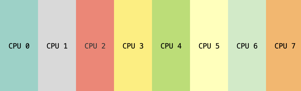 Column-wise sharding of tensor with 8 emulated devices.
There are various other ways to shard our tensor: we can split it along batch dimension or, even more, arrange our devices in 4x2 mesh and mesh both axes:
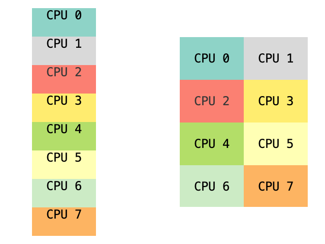 Some other ways to shard tensor.
Another way to place a tensor on devices that we need to look at before moving forward is tensor replication. Replicating tensor means that several devices will store their own copies of the whole tensor x:
1
2
replicated_x = jax.device_put(x, sharding.replicate(0))
visualize(replicated_x, color_map="Pastel2_r")
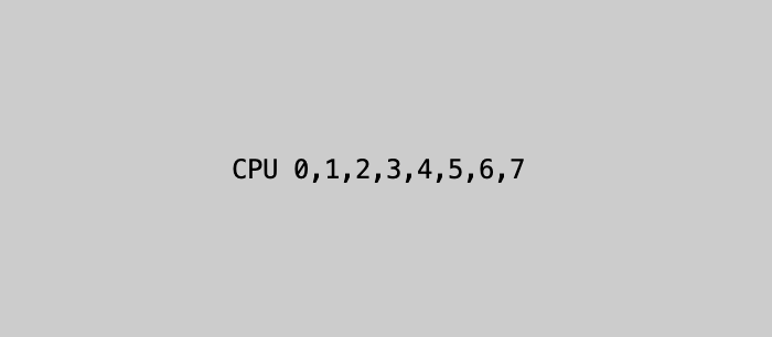 Device placement for replicated tensor $x$.
One can also combine sharding with replicating:
1
2
combined_x = jax.device_put(x, sharding.reshape(2, G // 2).replicate(0))
visualize(combined_x)
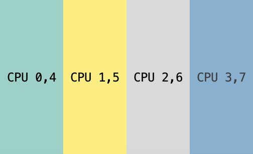 Device placement for sharded and replicated tensor $x$.
We will follow the similar way for visualization
Visualization of tensors locations. On the left side - tensor is split column-wise by 4 subtensors, each located on its designated device. On the right side - tensor is copied on 2 devices.
Parallel processing
Let’s create a simple feed-forward layer (FFN), which is one of the core components in modern LLMs. It consists of two linear layers and an activation function between them. If we omit bias and use ReLU as activation between layers, then FFN can be written as
\[\operatorname{FFN}(x) = \max(0, x\mathbf{W}_1)\mathbf{W}_2,\]where $x \in \mathbb{R}^{B \times d}$, $\mathbf{W}_1 \in \mathbb{R}^{d \times h}$ and $\mathbf{W}_2 \in \mathbb{R}^{h \times d}$. We will refer to $B$, $d$ and $h$ as to batch size, embedding and hidden dimensions respectively.
1
2
3
4
5
6
7
8
9
10
11
12
from jax import jit, random
from typing import NamedTuple
from jax._src.typing import ArrayLike

class Params(NamedTuple):
    w1: jnp.ndarray
    w2: jnp.ndarray

@jit
def ffn(x: jnp.array, params: Params):
    z = jnp.maximum(x @ params.w1, 0)
    return z @ params.w2
Let us also define additional mock functions for data sampling (both features and labels) and FFN weights initialization:
1
2
3
4
5
6
7
8
9
10
11
12
13
14
15
16
17
18
def init_ffn_weights(embed_dim: int, hidden_dim: int, rng: ArrayLike):
    '''
        Create FFN weights with Xavier initialization
    '''
    std = jnp.sqrt(2 / (embed_dim + hidden_dim))
    w1_key, w2_key = random.split(rng)
    w1 = std * random.normal(w1_key, (embed_dim, hidden_dim))
    w2 = std * random.normal(w2_key, (hidden_dim, embed_dim))
    return Params(w1, w2)

def sample_data(batch_size: int, embed_dim: int, rng):
    '''
        Create random features `x` and dependable random targets `y`
    '''
    x = random.normal(rng, (batch_size, embed_dim))
    w = random.normal(random.PRNGKey(1), (embed_dim, embed_dim))
    y = jnp.sin(x @ w)
    return x, y
Now we can run forward pass through FFN layer in Jax simply like this:
1
2
3
4
5
6
7
8
9
# set up toy example hyper-parameters
B, d, h = 16, 8, 32
# create random keys
data_key = random.PRNGKey(0)
weight_key = random.PRNGKey(42)

x, y = sample_data(B, d, data_key)
params = init_ffn_weights(d, h, weight_key)
y_pred = ffn(x, params)
Here x is stored on one single device and so is y_pred. Recall that x is basically a stack of B features with size d. It means that we can split this stack along batch dimension and send each part to its own device and process everything in parallel. And we already know how to implement that:
1
2
sharded_x = jax.device_put(x, sharding.reshape(G, 1))
visualize(ffn(sharded_x, params))
Data Parallelism
Data Parallel (DP) is a relatively simple strategy, but it allows scaling to large data batches: the training data is partitioned across $G$ distributed workers and fed to the model, which is replicated. The training process is done in parallel: dataloader spits out a batch of the total size $B$, then each worker computes activations, loss values $\ell$ and model gradients with its independent data split of size $S=\frac{B}{G}$. Gradients are then synchronized at the end of each training step before the weights update, so that all workers observe consistent model parameters throughout training.
Data Parallel strategy with 4 devices. Embedding and hidden dimensions $d$ and $h$ are equal to 2 and 4 respectively. Each device runs computations with its own separate shard of size $S$ equal to 5
Let’s build and example of a regression training loop with data parallelism. First, we build a deep neural network, consisting of $L$ FFN layers with residual connections (to prevent outputs degenerating to zeros due to ReLU activation). We also set up loss criteria and dataset and weights initialization functions.
1
2
3
4
5
6
7
8
9
10
11
12
13
14
15
16
17
18
19
20
21
22
23
24
25
26
27
28
29
30
31
32
33
@jit
def model(x: ArrayLike, params: Params) -> Array:
    for p in params:
        x += ffn(x, p)
    return x

@jit
def criterion(y_pred: ArrayLike, y_true: ArrayLike) -> float:
    return jnp.mean((y_pred - y_true) ** 2)

@jit
def loss_fn(params: Params, x: ArrayLike, y: ArrayLike) -> float:
    y_pred = model(x, params)
    return criterion(y_pred, y)

def create_dataset(num_samples: int, batch_size: int, embed_dim: int) -> Array:
    '''
        Create an array of samples (`x`, `y`)
    '''
    return jnp.array([
        sample_data(batch_size, embed_dim, random.PRNGKey(i))
        for i in range(num_samples)
    ])

def init_weights(embed_dim: int, hidden_dim: int, layer_num: int, rng: ArrayLike) -> list[Params]:
    '''
        Create weights for a stack of `layer_num` FFN layers
    '''
    layer_keys = random.split(rng, layer_num)
    return [
        init_ffn_weights(embed_dim, hidden_dim, layer_keys[l])
        for l in range(layer_num)
    ]
We’ve seen how to perform simple parallel operations manually, e.g. batching a simple FFN forward pass across several devices. JAX also supports automatic device parallelism: we can use jax.pmap to transform a function written for one device into a function that runs in parallel on multiple devices.
1
2
3
4
x = jnp.arange(G * d).reshape(G, d) # dummy sample
# replicate model weights
params = jax.tree_map(lambda p: jnp.tile(p, (G, 1, 1)), params)
visualize(jax.pmap(ffn, axis_name='G')(x, params))
Here’s how pmap works: ffn() takes data tensors of shape [B, ...] and computes the output of FFN layer on that batch. We want to spread the batch dimension across all available devices. To do that, we add a new axis. The arguments to the wrapped ffn() thus need to have shape [G, B/G, ...]. So, to call ffn(), we’ll need to reshape data batches so that what used to be batch is reshaped to [G, B/G, ...]. That’s what split() does below:
1
2
def split(arr: ArrayLike, num_sections: int=None, axis: int=0) -> Array:
    return jnp.array(jnp.split(arr, num_sections, axis=axis))
Additionally, we’ll need to replicate our model parameters, adding the G axis. This reshaping is how a pmapped function knows which devices to send which data.
With all that being said, we still need to send gradient information between the devices. For that, we can use special collective ops such as the jax.lax.p* ops psum, pmean, pmax, etc. In order to use the collective ops we must specify the name of the pmap-ed axis through axis_name argument, and then refer to it when calling the op. Here is a function update(), which runs forward and backward calculations, updates model parameters and all of it is done in parallel on different devices:
1
2
3
4
5
6
7
8
9
10
11
12
13
14
15
16
17
18
19
20
21
22
import functools

# Remember that the 'G' is just an arbitrary string label used
# to later tell 'jax.lax.pmean' which axis to reduce over. Here, we call it
# 'G', but could have used anything, so long as 'pmean' used the same.
@functools.partial(jax.pmap, axis_name='G')
def update(params: Params, x: ArrayLike, y: ArrayLike) -> Any:
    # Compute the gradients on the given minibatch (individually on each device)
    loss, grads = jax.value_and_grad(loss_fn)(params, x, y)

    # Combine the gradient across all devices (by taking their mean)
    grads = jax.lax.pmean(grads, axis_name='G')

    # Also combine the loss. Unnecessary for the update, but useful for logging
    loss = jax.lax.pmean(loss, axis_name='G')

    # Each device performs its own update, but since we start with the same params
    # and synchronise gradients, the params stay in sync
    LEARNING_RATE = 1e-3
    new_params = jax.tree_map(
       lambda param, g: param - g * LEARNING_RATE, params, grads)
    return new_params, loss
During the update step, we need to combine the gradients computed by each device – otherwise, the updates performed by each device would be different. That’s why we use jax.lax.pmean to compute the mean across the G axis, giving us the average gradient of the batch. That average gradient is what we use to compute the update.
Combining all together, we can now create a full train cycle with data parallel strategy:
1
2
3
4
5
6
7
8
9
10
11
12
13
14
15
16
17
18
19
20
def train_with_data_parallel(dataset, params, num_epochs):
    G = jax.local_device_count()
    # replicate model weights
    replicated_params = [
        jax.tree_map(lambda param: jnp.tile(param, (G, 1, 1)), p)
        for p in params
    ]
    for epoch in range(num_epochs):
        avg_loss = 0
        for (x, y) in tqdm(dataset, leave=False):
            # shard data batch
            x, y = split(x, G), split(y, G)
            replicated_params, loss = update(replicated_params, x, y)
            # note that loss is actually an array of shape [G], with identical
            # entries, because each device returns its copy of the loss
            # visualize(loss) will show [CPU 0, CPU 1, ..., CPU G]
            avg_loss += loss.mean().item()
        if (epoch + 1) % 5 == 0:
            print(f"Step {epoch + 1:3d}, loss: {avg_loss / dataset.shape[0]:.3f}")
    return replicated_params
We only need to set hyper-parameters, define training dataset and initialize weights to finally call the training function.
1
2
3
4
5
6
7
8
9
10
# set G = 4 devices
os.environ["XLA_FLAGS"] = '--xla_force_host_platform_device_count=4'

num_epochs = 50
num_samples = 500
B, d, h, L = 20, 2, 4, 16
dataset = create_dataset(num_samples, B, d)
print('Dataset size:', dataset.shape) # [N, 2, B, d]
params = init_weights(d, h, L, random.PRNGKey(42))
train_with_data_parallel(dataset, params, num_epochs)
And we can observe the process of our model being trained:
1
2
3
4
5
6
7
8
9
10
11
Dataset size: (500, 2, 20, 2)
Step   5, loss: 0.233
Step  10, loss: 0.184
Step  15, loss: 0.127
Step  20, loss: 0.117
Step  25, loss: 0.111
Step  30, loss: 0.106
Step  35, loss: 0.103
Step  40, loss: 0.100
Step  45, loss: 0.098
Step  50, loss: 0.097
The main problem with DP approach is that during the backward pass all the gradients must be transferred to the all other devices. For example, with $\mathbf{W}_1 \in \mathbb{R}^{d \times h}$ weight matrix in float32 $32 \cdot d \cdot h$ bits need to be sent between each pair of devices. The same amount is needed for $\mathbf{W}_2$. If we work in a multi-node setup with $v$ GBit/s of network card bandwidth, we’ll need
\[t = \frac{64 \cdot d \cdot h}{v \cdot 1024^3}\]seconds to send the gradients for FFN layer from one node to another (plus an additional overhead $\delta t$ that is neglected here). Given the substantial amount of data communication required in DP, a fast connection (interconnect) between computing devices is necessary. While DP may work for TPU device networks scaling up to pod levels, modern GPUs predominantly have fast interconnectivity only within a group of 8 devices hosted on the same system. Inter-GPU communication is considerably slower across separate hosts.
There is an example: imagine that we use data parallelism for LLM pretraining and we need to give a rough estimation of the time required for backward calculations. In GPT-3 the embedding size $d$ is $12 \cdot 1024$ with hidden size $h=4d$. Microsoft built a supercomputer exclusively for OpenAI with 10,000 GPUs and 400 GBit/s of network connectivity between nodes. Plugging in these numbers we get
\[t = \frac{64 \cdot 4 \cdot 12^2 \cdot 1024^2}{400 \cdot 1024^3} = 90\mbox{ms}\]just to transfer FFN gradients. Since there are 96 FFN layers in GPT-3, it’ll take about 9 seconds for this part of gradient synchronization. And this is just to send data from one node to another, while there might be dozens, hundreds or even thousands nodes with all-to-all communication cost growing quadratically. Easily we can see that data parallelism does not scale with size of the cluster and cannot be used in isolation for large models.
The described strategy above is also called Distributed Data Parallel (DDP) and it is different from PyTorch definition of data paralelism (also check out HuggingFace explanation). PyTorch version of DP helps to overcome slow intra-node connectivity by minimizing the amount of synchronized data and delegating a lot of data/gradient processing to one leading GPU. This, in turn, results in under-utilization of other devices.
Another common strategy for amortizing communication cost is gradient accumulation. We can run multiple forward and backward propagations and accumulate local gradients on each device in parallel before launching data synchronization and taking optimizer step. Additionally, performance can be improved by synchronizing the computed gradients for some tensors while simultaneously computing gradients for anothers.
Model parallelism
With the advent of large neural networks that do not fit on one device, the need to parallelize models has increased. This is especially true in the case of LLMs, whose number of parameters can exceed the already considerable amount of input data. To distribute computation and memory we can split the model across multiple devices and across multiple dimensions.
Tensor Parallelism
The idea of sharding, the way it was applied to data tensors, can be used in a similar way with respect to the model weights. We can divide each tensor $\mathbf{W}$ into chunks distributed across multiple devices, so instead of having the whole tensor reside on a single device, each shard of the tensor resides on its own accelerator. Each part gets processed separately in parallel on different devices and after processing the results are synced at the end of the step.
Such strategy is called Tensor Parallel (TP) or horizontal parallelism, as the splitting happens on horizontal level (we will get to the vertical/pipeline parallelism later). A simple and efficient way to parallelize FFN calculations was proposed in Megatron-LM paper. Let’s represent matrices $\mathbf{W}_1$ and $\mathbf{W}_2$ as concatenation of $G$ sub-tensors along rows and columns respectively:
\[\mathbf{W}_1 = \begin{pmatrix} \color{#8ED3C7}{\mathbf{W}_1^1} & \color{#FDBFB9}{\mathbf{W}_1^2} & \cdots & \color{#FDB462}{\mathbf{W}_1^G} \end{pmatrix}, \quad \mathbf{W}_2 = \begin{pmatrix} \color{#8ED3C7}{\mathbf{W}_2^1} \\ \color{#FDBFB9}{\mathbf{W}_2^2} \\ \vdots \\ \color{#FDB462}{\mathbf{W}_2^G} \end{pmatrix}\]with $\mathbf{W}_1^k \in \mathbb{R}^{d \times \frac{h}{G}}$, $\mathbf{W}_2^k \in \mathbb{R}^{\frac{h}{G}\times d}$ for $k = 1, \dots, G$. Then with $x$ replicated over devices we can perform sub-tensors multiplications in parallel:
\[x\mathbf{W}_1=\begin{pmatrix} x\color{#8ED3C7}{\mathbf{W}_1^1} & x\color{#FDBFB9}{\mathbf{W}_1^2} &\cdots & x\color{#FDB462}{\mathbf{W}_1^G} \end{pmatrix}\]and for $z = \max(x\mathbf{W}_1, 0)$ we have
\[z\mathbf{W}_2=z {\color{#8ED3C7}{\mathbf{W}_2^1}} + z {\color{#FDBFB9}{\mathbf{W}_2^2}} + \cdots + z {\color{#FDB462}{\mathbf{W}_2^G}}.\]The model weights on different devices do not overlap, and the only communication between devices occurs at the end of the FFN layer when we need to sum all the outputs. We can already see the advantage of TP over DP here: computational costs for each device decreases drastically with growing number of devices. On the other hand, the deficiency of TP is that the input data is replicated, so that the batch size per device is now equal to the total batch size. Hence if we are restricted by GPU memory we have to reduce our $B$. Otherwise, we can increase our $S$ by a factor of $G$ to keep up with the same batch size $B=S \times G$ as in DP strategy.
Tensor Parallel strategy with batch size $B$ set to 5. Each device stores its own part of model weights. Activations are aggregated after each FFN layer.
1
2
3
4
5
6
7
8
9
10
11
12
13
14
15
16
17
def train_with_tensor_parallel(dataset, params, num_epochs):
    G = jax.local_device_count()
    sharded_params = [
        Params(w1=split(p.w1, num_sections=G, axis=1),
               w2=split(p.w2, num_sections=G, axis=0))
        for p in params
    ]
    for epoch in range(num_epochs):
        avg_loss = 0
        for (x, y) in tqdm(dataset, leave=False):
            # replicate data batch
            x, y = jnp.array([x] * G), jnp.array([y] * G)
            sharded_params, loss = update(sharded_params, x, y)
            avg_loss += loss.mean().item()
        if (epoch + 1) % 5 == 0:
            print(f"Step {epoch + 1:3d}, loss: {avg_loss / dataset.shape[0]:.3f}")
    return sharded_params
Since in TP the size of synchronized weights equals to the batch size $B$ multiplied by embedding size $d$, when we operate with float32, each device sends $32 \cdot d \cdot B$ bits to each other device. Thus, the amount of memory transfer between each pair of devices is $\mathcal{O}(dh)$ for DP versus $\mathcal{O}(dB)$ for TP. We can conclude, that DP is a preferable strategy for small networks (e.g. model can fit onto one device), while TP works better with larger models and smaller batches.
Hybrid data and model tensor parallelism
It is common to mix both data and tensor parallelism for large scale models. With a total of $G=\operatorname{TP}\times \operatorname{DP}$ devices, each device stores $\frac{B}{\operatorname{DP}}$ embedding vectors and $\frac{h}{\operatorname{TP}}$ of both the weights and intermediate activations.
1
2
3
4
5
6
7
8
9
10
11
12
13
14
15
16
17
18
19
20
21
def train_with_hybrid_parallel(dataset, params, num_epochs, DP, TP):
    sharded_params = [
        Params(w1=split(p.w1, num_sections=TP, axis=1),
               w2=split(p.w2, num_sections=TP, axis=0))
        for p in params
    ]
    hybrid_params = [
        jax.tree_map(lambda param: jnp.tile(param, (DP, 1, 1)), p)
        for p in sharded_params
    ]
    for epoch in range(num_epochs):
        avg_loss = 0
        for (x, y) in tqdm(dataset, leave=False):
            # shard and then replicate data batch
            x, y = split(x, DP), split(y, DP)
            x, y = jnp.repeat(x, TP, axis=0), jnp.repeat(y, TP, axis=0)
            hybrid_params, loss = update(hybrid_params, x, y)
            avg_loss += loss.mean().item()
        if (epoch + 1) % 5 == 0:
            print(f"Step {epoch + 1:3d}, loss: {avg_loss / dataset.shape[0]:.3f}")
    return hybrid_params
Pipeline Parallelism
Suppose our neural network, a stack of $L$ FFN layers, is so deep, that it doesn’t fit on a single device. This scenario is practical because a common way to scale up models is to stack layers of the same pattern. It might feel straightforward for us to split our model by layer and that is what Pipeline Parallel (PP) strategy does. It splits up the model weights vertically, so that only a small group of consecutive layers of the model are placed on a single device.
Naive Pipeline Parallel strategy. Each stage represent forward/backward pass through its own sequence of $\frac{L}{G}$ FFN layers on each device. It can be seen that running every data batch through multiple workers with sequential dependencies leads to large idle bubbles and severe under-utilization of computation resources.
To implement naive PP strategy in Jax we just have to place layers to their corresponding devices and whenever the data goes in each layer it must be switched to the same device.
Clearly, the main disadvantage of this type of parallelization is that all but one device is idle at any given moment. In addition, at the end of each stage there is a serious communication overhead for transferring data between devices. To reduce idling problem we have to explore other approaches.
Pipeline Parallel reduced to tensor sharding
Since our model only consists of $L$ equal (not shared) layers, when we split it vertically, our pipelining scenario looks like $G$ stages of the same subcomputation except for having different weight values. The similar picture we could’ve seen in TP strategy - every device is doing the same operations but with different operands.
Let’s reorganize the way we look at our model architecture. If we stack weights from different stages and represent them all together as tensors $\mathbf{W}_1 \in \mathbb{R}^{G \times d \times h}$ and $\mathbf{W}_2 \in \mathbb{R}^{G \times h \times d}$ in each FFN layer, we can shard them across stacked axis, so that these stages can be run in parallel, but with different batches. Although, $k$-th stage still have to wait until output activations from $(k-1)$-th stage are calculated and transferred to the $k$-th device. It means that first $k$ runs for $k$-th stage must be done with emulated input data, e.g. filled with zeros or random values.
Pipeline Parallel inference with inter-batch parallelism. White cells represent zero-paddings.
The extra iterations are equivalent to the bubbles that describe the idle time due to data dependency, although the waiting devices compute on padded data instead of being idle. One can notice that if we split our batch into multiple micro-batches and enable each stage worker to process one micro-batch simultaneously, idle bubbles become much smaller, compared to naive PP.
1
2
3
4
5
6
7
8
9
10
11
12
13
14
15
16
17
18
19
20
21
22
23
24
25
26
27
28
29
30
31
32
33
34
def stack_stage_weights(params: list[Params]) -> list[Params]:
    '''
        Stack G stages, each containing L/G FFN layers
    '''
    L = len(params)
    G = jax.local_device_count()
    assert L % G == 0, f"Number of layers {L} must be divisible by number of stages {G}"
    stage_layers = L // G
    out_params = []
    for l in range(stage_layers):
        w1 = jnp.stack([params[l + g * stage_layers].w1 for g in range(G)])
        w2 = jnp.stack([params[l + g * stage_layers].w2 for g in range(G)])
        out_params.append(Params(w1, w2))
    return out_params

def pipeline_inference(params: list[Params], x: ArrayLike, M: int) -> Array:
    '''
        Split input batch to M micro-batches and run PP forward pass
    '''
    B = x.shape[0]
    micro_batch_size = B // M
    # re-organize weights
    params = stack_stage_weights(params)
    # split input data to micro-batches
    x = split(x, M)
    # create shifting buffer
    state = jnp.zeros((G, micro_batch_size, d))
    y_pred = []
    for i in range(M + G - 1):
        from_prev_stage = jnp.concatenate([jnp.expand_dims(x[i], 0), state[:-1]])
        state = jax.pmap(model)(from_prev_stage, params)
        if i >= G - 1: # first micro-batch has passed through the last stage
            y_pred.append(state[-1])
    return jnp.array(y_pred).reshape(B, d)
This is the main idea in GPipe (Huang et al. 2019) paper. During training stage, backward calculations are scheduled in reverse order. Gradients from multiple micro-batches are aggregated and applied synchronously at the end, which guarantees learning consistency and efficiency. Given $M$ evenly split micro-batches, the idle time is $O \big( \frac{G - 1}{M + G - 1} \big)$ amortized over the number of micro-steps.
To reduce memory footprint gradient checkpointing can be applied, meaning that during forward computation, each device only stores output activations at the stage boundaries. During the backward pass on $k$-th device the $k$-th stage forward pass re-computes the rest of activations. While it doubles time, required for forward calculations, it helps to reduce peak activation memory requirement to $O \big(B + \frac{L}{G} \times \frac{B}{M}\big)$. In comparison, memory requirement without PP and gradient checkpointing would be $\mathcal{O}(B \times L)$, since computing the gradients requires both the next layer gradients and the cached activations.
Expert Parallelism
With Mixture-of-Experts (MoE) models, different sub-networks (FFN layers in our case) or so-called “experts” specialize in different parts of the input space. For example, in a language model, some experts may specialize in grammar while others focus on semantic understanding. The key to a mixture of experts is having a gating network $\mathcal{G}$ that assigns different parts of each input to the most relevant experts.
During training, only the experts assigned to a given input have their parameters updated. This sparse update allows mixture of experts models to scale to thousands or even tens of thousands of experts. Each expert can be updated in parallel by a different set of accelerators without heavy communication overhead.
Mixture of Expert Routing
MoE layer was proposed by Shazeer et al. (2017). It takes a token representation $x$ and then routes it through gating network $\mathcal{G}$ to determined experts. Say, we have $E$ experts in total, then the output of the MoE layer $y$ is the linearly weighted combination of each expert’s output by the gate value
\[y = \sum_{i=1}^E \mathcal{G}(x)_i \cdot \operatorname{FFN}_i(x).\]The simple choice of gating function is to create trainable weight matrix $\mathbf{W}_G$ to produce logits, which are normalized via a softmax distribution over the available experts at that layer:
\[\mathcal{G}(x)=\operatorname{softmax}(x\mathbf{W}_{\text{G}}).\]1
2
def dense_gating(x: ArrayLike, gate_params: ArrayLike) -> Array:
return jax.nn.softmax(x @ gate_params)
However, this choice raises two problems:
- MoE layer with dense control vector $\mathcal{G}(x)$ requires computation of all $E$ experts, even those whose impact to the output may be negligible. It would be more efficient if we didn’t have to compute $\operatorname{FFN}_i(x)$ when $\mathcal{G}(x)_i=0$.
- Self-reinforcing effect: gating network might favor a few strong experts everytime, leaving the rest of the layers redundant.
To overcome these issues we introduce sparsity through $\operatorname{topk}$ function and noise via standard Gaussian variable $\epsilon \sim \mathcal{N}(0, 1)$. The amount of noise per component is controlled by a second trainable weight matrix $\mathbf{W}_{\text{noise}}$. Modified gating function would like like this:
\[\mathcal{G}(x)=\operatorname{softmax}(\operatorname{topk}(H(x), k)),\]where
\[H(x)_i = (x\mathbf{W}_{\text{G}})_i + \epsilon \cdot \operatorname{softplus}(x \mathbf{W}_{\text{noise}})_i\]and
\[\operatorname{topk}(v, k)_i = \begin{cases} v, & \text{if } v_i \text{ is in top } k \text{ elements of } v \\ -\infty, & \text{otherwise.} \end{cases}\]1
2
3
4
5
6
7
8
9
10
11
12
13
14
15
16
17
18
19
20
21
22
23
24
25
26
27
28
29
30
31
32
33
def scatter(input: ArrayLike, dim: int, index: ArrayLike, src: int) -> Array:
'''
Scatter function analogous to PyTorch `scatter_`
'''
idx = jnp.meshgrid(*(jnp.arange(n) for n in input.shape),
sparse=True,
indexing='ij')
idx[dim] = index
return input.at[tuple(idx)].set(src)
def index_to_mask(index: ArrayLike, input_shape: tuple) -> Array:
'''
Transform given indices to mask of input shape,
where mask[index] = True and False otherwise
'''
zeros = jnp.zeros(input_shape, dtype=bool)
return scatter(zeros, 1, index, True)
def sparse_gating(x: ArrayLike,
gate_params: ArrayLike,
topk: int,
noise_weights: ArrayLike=None,
rng: ArrayLike=None):
h = x @ gate_params
if noise_weights is not None:
assert rng is not None, "Random seed is required to use noisy gating"
eps = random.normal(rng, h.shape)
noise = eps * jax.nn.softplus(x @ noise_weights)
h += noise
_, top_k_ids = jax.lax.top_k(h, topk)
mask = index_to_mask(top_k_ids, h.shape)
h = jnp.where(mask, h, -jnp.inf)
return jax.nn.softmax(h)
To help load-balancing and to avoid collapse to using a small number of experts an auxiliary importance loss was proposed. Let’s define an importance of an expert $i$ relative to the batch $\mathcal{B}$ as batchwise sum of the gate values for that expert: $\sum_{x \in \mathcal{B}} \mathcal{G}(x)_i$. Importance loss minimizes the squared coefficient of variation of importance over experts:
\[\ell_{\text{aux}}(\mathcal{B}) = \operatorname{CV} \big( \sum_{x \in \mathcal{B}} \mathcal{G}(x) \big)^2.\]Such constraint encourages all experts to have equal importance values.
Another important detail is that since each expert network receives only a portion of the training samples, we should try to use as large a batch size as possible in MoE. To improve the throughput MoE can be combined with DP strategy.
GShard
Additional experts increase the amount of model parameters significantly. Basically MoE layer requires $E$ times more parameters than a single FFN layer (plus gating tensor $\mathbf{W}_{\text{G}}$). But what if we had each expert reside on its own device? GShard (Lepikhin et al., 2020) uses the idea of sharding across expert dimension to scale up the MoE transformer model up to 600B parameters. The MoE transformer replaces every other FFN with a MoE layer. All MoE layers are different across devices, while other layers are duplicated.
 Illustration of scaling of Transformer Encoder with MoE Layers. (a) The encoder of a standard Transformer model is a stack of self-attention and feed forward layers interleaved with residual connections and layer normalization. (b) By replacing every other feed forward layer with a MoE layer, we get the model structure of the MoE Transformer Encoder. (c) When scaling to multiple devices, the MoE layer is sharded across devices, while all other layers are replicated.
Authors chose to let each token $x$ dispatched to at most two experts. Besides that, there are several improvements for the gating function in GShard:
- To ensure that expert load is balanced, the number of tokens processed by one expert is restricted by threshold $C$ named expert capacity. If a token $x$ is routed to an expert that has reached its capacity, the token be considered overflowed and gating output $\mathcal{G}(x)$ degenerates into a zero vector. Such token has its representation $x$ passed on to the next layer via residual connection.
- Local group dispatching: $\mathcal{G}(\cdot)$ partitions all tokens in a training batch evenly into $G$ groups, each of size $S$ and the expert capacity is enforced on the group level.
- Random routing: since MoE layer output $y$ is a weighted average, if the 2nd best expert gating weight is small enough, we can skip expert computation. To comply with the capacity constraint, token is dispatched to the expert with with a probability proportional to its weight.
- Auxiliary loss to avoid experts under-utilization is modified. Let $p(x)$ be dense gating function:
Also let $f_i$ be the fraction of tokens in a group $\mathcal{S}$ dispatched to expert $i$:
\[f_i = \frac{1}{S} \sum_{x \in \mathcal{S}} \mathbb{1}_{ \lbrace \operatorname{argmax} \mathcal{G}(x) = i \rbrace },\]The goal is to minimize mean squared ratio of tokens per expert: $\frac{1}{E} \sum_{i=1}^E f_i^2$. But since this value is derived from $\operatorname{topk}$ function, it’s non-differentiable, so authors propose to use mean gating weights as differentiable approximation:
\[\bar{p}_i = \frac{1}{S} \sum_{x \in \mathcal{S}} p(x)_i \approx f_i.\]Then $\ell_{\text{aux}} = \sum_{i=1}^E f_i \cdot \bar{p}_i$.
Switch Transformer
Switch Transformer scales the model size even more, up to 1.6 trillion parameters, by replacing FFN layer with a sparse MoE layer in which each input is routed to only one expert network. Authors refer to such routing strategy as a Switch layer. Similar to how it is done in GShard each expert has its capacity $C$, which depends on batch size $B$ and number of experts $E$ by formula
\[C = \frac{B}{E} \cdot c,\]where $c$ is a capacity factor. A capacity factor greater than 1.0 creates additional buffer to accommodate for when tokens are not perfectly balanced across experts.
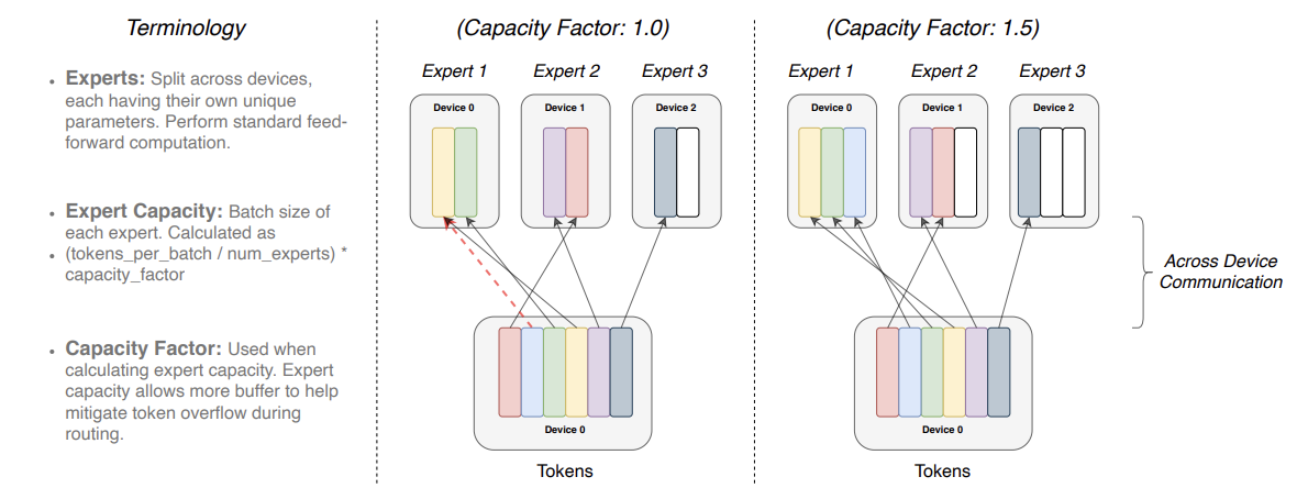 Each token $x$ is routed to the expert with the highest router probability $p(x)$, but each expert has a fixed batch size $C$. Smaller capacity factor can lead to experts overflow, while larger factor increases computation and communication costs.
Let’s dive into implementation details and describe step-by-step how to combine Switch layer with Data Parallel strategy.
- Switch Transformer is allocated on $G$ devices, which will also correspond to the number of experts $E$. For each token per device gating function locally computes assignments to the experts.
1
2
3
4
5
6
7
8
9
10
11
# Probabilities for each token of what expert it should be sent to.
# gating_probs shape: [G, S, E]
gating_probs = jax.nn.softmax(x @ gate_params)

# Get the top−1 expert for each token.
# expert_gate is the probability from the gating to top-1 expert
# expert_index is what expert each token is going to be routed to
# expert_gate shape: [G, S]
# expert_index shape: [G, S]
expert_gate, expert_index = jax.lax.top_k(gating_probs, 1)
expert_gate, expert_index = expert_gate.squeeze(), expert_index.squeeze()
- The output is a dispatch mask, a 4-D binary tensor of shape $[G, S, E, C]$, which is partitioned across the first dimension and determines expert assignment. On each device $g$ for each token $s$ 2-D slice of dispatch mask contains at most one non-zero element.
1
2
3
4
5
6
7
8
9
10
11
12
13
14
15
16
17
18
19
20
21
22
23
# expert_mask shape: [G, S, E]
expert_mask = jax.nn.one_hot(expert_index, num_classes=gating_probs.shape[2])

# Experts have a fixed capacity C, ensure we do not exceed it.
# Construct the batch indices, to each expert, with position in expert
# make sure that not more that C examples can be routed to each expert.
position_in_expert = jnp.cumsum(expert_mask, axis=1) * expert_mask

# Keep only tokens that fit within expert capacity.
expert_mask_trunc = expert_mask * jnp.less(position_in_expert, expert_capacity)
expert_mask_flat = jnp.sum(expert_mask_trunc, axis=2)

# Mask out the experts that have overflowed the expert capacity.
expert_gate *= expert_mask_flat

# combine_tensor used for combining expert outputs and scaling with gating probability.
# combine_tensor shape: [G, S, E, C]
expert_capacity_int = int(jnp.ceil(expert_capacity))
combine_tensor = (expert_gate[..., None, None] *
                  expert_mask[..., None] *
                  jax.nn.one_hot(position_in_expert, num_classes=expert_capacity_int))
combine_tensor = combine_tensor[..., 1:] # cut 0-dimension which is always 0s
dispatch_mask = combine_tensor.astype(bool)
- This mask is then used to do a gather via Einstein summation with the partitioned input tensor $x$ of size $[G, S, d]$, resulting in the final tensor of shape $[E, G, C, d]$, which is sharded across second dimension. Because each device has its own expert, we do an all-to-all communication of size $[E, C, d]$ to now shard the $E$-dimension instead of the $G$-dimension.
1
2
3
4
5
6
7
8
9
10
11
# Matmul with large boolean tensor to assign tokens to the correct expert.
# device layout: [G, 1, 1], −> [1, G, 1, 1]
# expert inputs shape: [E, G, C, d]
expert_inputs = jnp.einsum("GSEC,GSd->EGCd", dispatch_mask, x)

# All−to−All communication. Cores split across G and now we want to split
# across E. This sends tokens, routed locally, to the correct expert now
# split across different cores.
# device layout: [1, G, 1, 1] −> [G, 1, 1, 1]
sharding = PositionalSharding(jax.devices())
expert_inputs = jax.device_put(expert_inputs, sharding.reshape(G, 1, 1, 1))
- Next, we run experts computation with re-sharded inputs and perform all-to-all communication once again to shard expert outputs back along $G$ dimension.
1
2
3
4
5
6
7
8
9
10
# Standard FFN computation, where each expert has
# its own unique set of parameters.
# Total unique parameters created: E * (d * h * 2).
# expert_outputs shape: [E, G, C, d]
expert_outputs = ffn(expert_inputs, ffn_params)

# All−to−All communication. Cores are currently split across the experts
# dimension, which needs to be switched back to being split across num cores.
# device layout: [G, 1, 1, 1] −> [1, G, 1, 1]
expert_outputs = jax.device_put(expert_outputs, sharding.reshape(1, G, 1, 1))
- And finally, to get $y$, we average expert outputs based on gating probabilities:
1
2
3
4
5
# Convert back to input shape and multiply outputs of experts by the gating probability
# expert_outputs shape: [E, G, C, d]
# expert_outputs_combined shape: [G, S, d]
# device layout: [1, G, 1, 1] −> [G, 1, 1]
expert_outputs_combined = jnp.einsum("EGCd,GSEC->GSd", expert_outputs, combine_tensor)
A schematic representation of top-1 expert parallel dispatching with data parallel and batch size per device $S=5$. Number of experts $E$ is equal to the number of devices $G$ and capacity factor $c$ is set to 2 (therefore expert capacity $C = \frac{S}{E} \cdot c = 2.5$). Any white cell represents zero element. Vectors associated with the first token placed on GPU-1 (initially) are shaded as an example so that the flow of elements in the image can be easily followed. Note that the embedding of this token was dispatched to the last expert by
Gating and therefore put to the last device accordingly.
The auxiliary loss $\ell_{\text{aux}}$ is similar to GShard, except that $f_i$ is derived through dense gating function and aggregated over whole batch:
\[f_i = \frac{1}{B} \sum_{x \in \mathcal{B}} \mathbb{1}_{ \lbrace \operatorname{argmax} \mathcal{p}(x) = i \rbrace }.\]The same goes for $\bar{p}_i$.
1
2
3
4
5
6
7
8
9
10
11
12
13
14
15
16
17
18
19
20
21
22
23
def load_balance_loss(gating_probs, expert_mask):
    '''
        Calculate load−balancing loss to ensure diverse expert routing.
    '''
    # gating probs is the probability assigned for each expert per token
    # gating probs shape: [G, S, E]
    # expert index contains the expert with the highest gating
    # probability in one−hot format
    # expert mask shape: [G, S, E]
    # For each core, get the fraction of tokens routed to each expert
    # density_1 shape: [G, E]
    density_1 = jnp.mean(expert_mask, axis=1)
    # For each core, get fraction of probability mass assigned to each expert
    # from the router across all tokens.
    # density_1_proxy shape: [G, E]
    density_1_proxy = jnp.mean(gating_probs, axis=1)
    # density_1 for a single device: vector of length E that sums to 1.
    # density_1_proxy for a single device: vector of length E that sums to 1.
    # Want both vectors to have uniform allocation (1/E) across all E elements.
    # The two vectors will be pushed towards uniform allocation when the dot product
    # is minimized.
    loss = jnp.mean(density_1_proxy * density_1) * (density_1.shape[-1] ** 2)
    return loss
Full code for Switch Layer can be found here.
Mixtral of Experts
Recently an open-source language model called Mixtral 8x7B was introduced in Mixture of Experts paper and is claimed to outperform Llama-2 70B and GPT-3.5 on many benchmarks. As the name suggests, inference requires running only through 7B parameters, which is possible thanks to 8 distinct experts for each layer. For Mixtral 8x7B authors use deterministic sparse gating function, routing to top 2 experts:
\[\mathcal{G}(x) = \operatorname{softmax}(\operatorname{topk} (x\mathbf{W}_{\text{G}}, 2)).\]Another key point is that the SwiGLU layer is chosen as the expert function. It was introduced by Noam Shazeer in GLU Variants Improve Transformers and has two main differences from standard FFN layer. The first one is Swish (also called SiLU) activation function instead of ReLU:
\[\operatorname{Swish}(x) = x \sigma (x) = \frac{x}{1+e^{-x}}.\]The second one is the gating mechanism, Gated Linear Unit (GLU), introduced by Dauphin et al., 2016:
\[\operatorname{SwiGLU}(x) = \big(\operatorname{Swish}(x \mathbf{W}_1) \otimes x \mathbf{V} \big)\mathbf{W}_2,\]where $\otimes$ is the element-wise product between matrices.
1
2
3
4
5
6
7
8
9
10
class SwiGLUParams(NamedTuple):
    w1: jnp.ndarray
    w2: jnp.ndarray
    v:  jnp.ndarray

@jit
def swiglu(x: ArrayLike, params: SwiGLUParams) -> Array:
    y = x @ params.v
    z = jax.nn.swish(x @ params.w1)
    return (z * y) @ params.w2
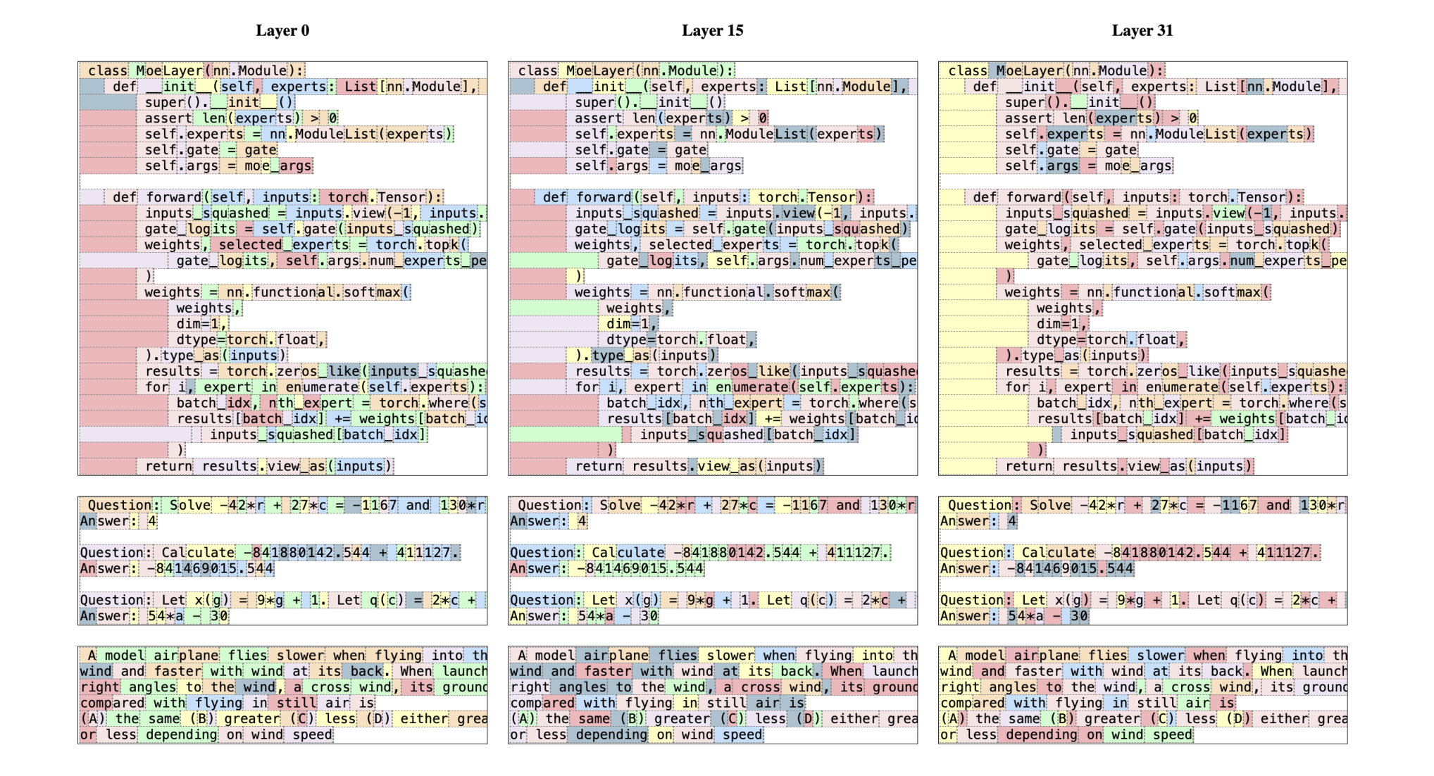 Routing analysis: each token is colored with the first expert choice in Mixtral 8x7B. Authors notice that the selection of experts appears to be more aligned with the syntax rather than the domain, especially at the initial and final layers.
Strategies worth considering but beyond the scope of this post
Zero Redundancy Optimizer (ZeRO) - it also performs sharding of the tensors somewhat similar to TP, except the whole tensor gets reconstructed in time for a forward or backward computation, therefore the model doesn’t need to be modified. It also supports various offloading techniques to compensate for limited GPU memory.
Fully sharded data parallel (FSDP) - is a type of data parallel training, but unlike traditional DP strategy, which maintains a per-GPU copy of a model’s parameters, gradients and optimizer states, it shards all of these states across data parallel workers and can optionally offload the sharded model parameters to CPUs.
Conclusion
Training ever-larger neural networks requires creative parallelization techniques to distribute computation and memory efficiently across accelerators. In this post, we explored some of the predominant strategies used today like data, tensor, pipeline, and mixture-of-experts parallelism.
While simple data parallelism can work for smaller models, combining it with model parallel approaches becomes essential to scale up to the massive architectures used in LLMs. Each strategy makes tradeoffs between computation efficiency, communication overheads, and implementation complexity.
Hybrid schemes are often needed in practice, tailored to optimize parallelism for a specific model architecture. As models continue growing in size, new innovations in efficient distributed training will be crucial to unlock further breakthroughs in AI. The insights from this post can guide decisions on parallelization strategies when training large neural networks.
Sources:
- Parallelization with Jax
- Data/model parallel strategies:
- Megatron-LM (Shoeybi et al. 2020)
- Using DeepSpeed and Megatron to Train Megatron-Turing NLG 530B (Smith et al. 2022)
- GSPMD: General and Scalable Parallelization for ML Computation Graphs (Xu et al. 2021)
- GPipe: Easy Scaling with Micro-Batch Pipeline Parallelism (Huang et al. 2019)
- How to Parallelize Deep Learning on GPUs.
- Mixture of Experts: