Building Aligned Intelligence System. Part II. Improving Large Language Models
In this post we will look at different techniques for steering LLMs behaviour to get desired outcomes, starting with some basic general principles such as writing a good prompt and ending with fine-tuning and augmenting models with external knowledge. Methods discussed in this post are mainly aimed at improving LLMs reliability and ensuring the consistency and factual accuracy of their outputs.
Prompt design
Smart prompt design essentially produces efficient context that can lead to desired completion. Such approach is important, because it does not require to change model weights and with a single model checkpoint one can perform many tasks. The general advice for writing a smart prompt is to start simple and iteratively adding more elements and context as you aim for better results.
Although some of the techniques are specific to certain types of problems, many of them are built upon general principles that can be applied to a wide range of tasks.
- Give specific instructions. If you want it to say “I don’t know” when it doesn’t know the answer, tell it ‘Say “I don’t know” if you do not know the answer.’
- Split complex tasks into simpler subtasks.
- Supply high quality and diverse examples.
- Generate multiple possible answer, ask for justifications and then pick the best one.
- Prompt the model to explain before answering. Ask it to write down the series of steps explaining its reasoning.
Chain-of-Thought
In previous part we saw such techniques as zero-shot, when user gives a direct instruction, and few-shot, when instruction is followed by examples in the prompt. But this simple methods could be still unreliable on tasks that require reasoning abilities. As an example, if you simply ask text-davinci-002 (GPT-3.5 model trained with SFT) the arithmetic problem, in most cases the answer will be wrong.
Standard few-shot example:
Q: Roger has 5 tennis balls. He buys 2 more cans of tennis balls. Each can
has 3 tennis balls. How many tennis balls does he have now?
A: The answer is 11.

Q: A juggler can juggle 16 balls. Half of the balls are golf balls, and half
of the golf balls are blue. How many blue golf balls are there?
A:
The answer is 8.
A technique known as chain-of-thought (CoT) introduced in Wei et al. (2022) is to prompt the model to explain step-by-step how it arrives at an answer.
CoT few-shot example:
Q: Roger has 5 tennis balls. He buys 2 more cans of tennis balls. Each can
has 3 tennis balls. How many tennis balls does he have now?
A: Roger started with 5 balls. 2 cans of 3 tennis balls each is 6 tennis balls.
5 + 6 = 11. The answer is 11.

Q: A juggler can juggle 16 balls. Half of the balls are golf balls, and half
of the golf balls are blue. How many blue golf balls are there?
A:
The juggler can juggle 16 balls. Half of the balls are golf balls. So there are
16 / 2 = 8 golf balls. Half of the golf balls are blue. So there are 8 / 2 = 4
blue golf balls. The answer is 4.Tests with PaLM 540B on GSM8K benchmark have shown that chain-of-thought outperforms few-shot prompting by a large margin: 57% solving rate on math problems, compared to near 18% with standard prompting. In addition to math problems, CoT also lifted performance on questions related to sports understanding, coin flip tracking, and last letter concatenation.
CoT enables complex reasoning capabilities, but it comes with a price: the increase in both latency and cost due to the increased number of input and output tokens. Also, most prompt examples are task-specific and require extra effort to generate. A recent technique, called zero-shot CoT (Kojima et al. 2022), simplifies CoT by essentially adding “Let’s think step by step” to the original prompt without providing any examples:
Zero-shot CoT example:
Q: A juggler can juggle 16 balls. Half of the balls are golf balls, and half
of the golf balls are blue. How many blue golf balls are there?
A: Let’s think step by step.
There are 16 balls in total. Half of the balls are golf balls. That means that
there are 8 golf balls. Half of the golf balls are blue. That means that there
are 4 blue golf balls.On GSM8K benchmark the “Let’s think step by step” trick raised solving rate up to 41% with InstructGPT. Similar magnitudes of improvements have been acheived with PaLM 540B as well. At the same time, while this trick works on math problems, it’s not effective in general. The authors found that it was most helpful for multi-step arithmetic problems, symbolic reasoning problems, strategy problems, and other reasoning problems. It didn’t help with simple math problems or common sense questions, and presumably wouldn’t help with many other non-reasoning tasks either.
Also, if you apply this technique to your own tasks, don’t be afraid to experiment with customizing the instruction. “Let’s think step by step” is rather generic prompt, so you may find better performance with instructions that hew to a stricter format customized to your use case.
Self-consistency
The idea of self-consistency proposed by Wang et al. (2022) is to sample multiple, diverse reasoning paths through few-shot CoT, and use the generations to select the most consistent answer. There are generally different thought processes for the same problem (e.g. different ways to prove the same theorem), and the output decision can be more faithful by exploring a richer set of thoughts. The output response can be picked either by majority vote, or by language model itself.
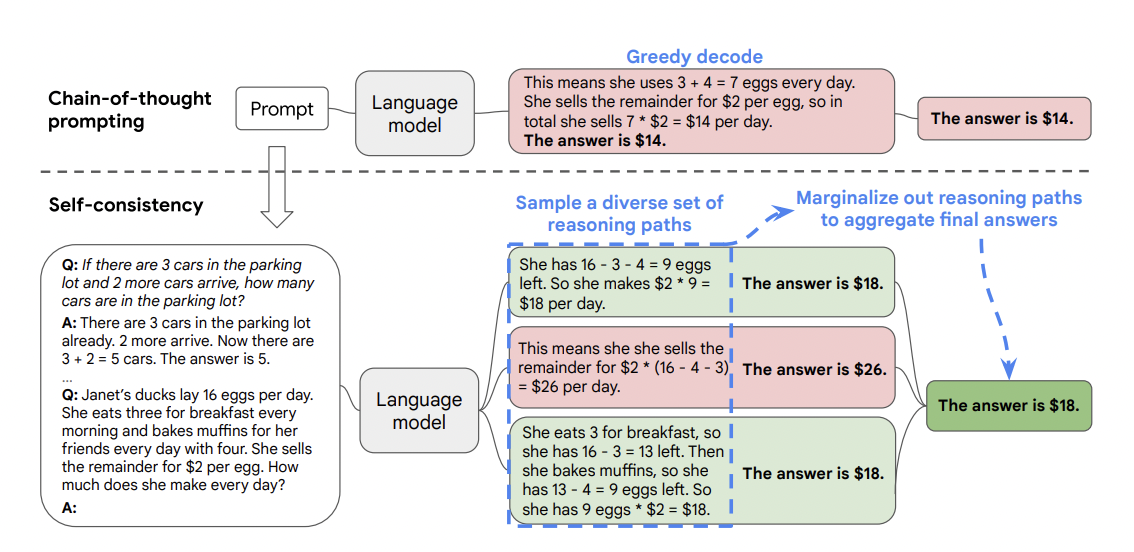 The self-consistency method contains three steps: (1) prompt a language model using chain-of-thought (CoT) prompting; (2) replace the “greedy decode” in CoT prompting by sampling from the language model’s decoder to generate a diverse set of reasoning paths; and (3) marginalize out the reasoning paths and aggregate by choosing the most consistent answer in the final answer set.
Self-consistency technique helps to boost the performance of CoT prompting on tasks involving arithmetic and commonsense reasoning. In particular, on arithmetic tasks self-consistency method applied to PaLM 540B and GPT-3 gave an increase in accuracy up to 17.9% compared to CoT-prompting, surpassing many SoTA solutions. On GSM8K benchmark code-davinci-002 (GPT 3.5 model optimized for code-completion tasks) with self-consistency reached 78%.
Although this technique is simple to implement, it can be costly. Remember, that generating a set of N answers will increase your costs N times. Another limitation is that the “most frequent” heuristic only applies when the output space is limited (e.g. multi-choice QA).
Tree of Thoughts
Simple prompting techniques can fall short in tasks that require exploration, strategic lookahead, or where initial decisions play a pivotal role. To overcome these challenges Yao et el. (2023) proposed Tree of Thoughts (ToT), a framework that generalizes over chain-of-thought prompting and encourages exploration over thoughts1. ToT allows LLMs to perform deliberate decision making by searching over multiple different reasoning paths and self-evaluating choices to decide the next course of action, as well as looking ahead or backtracking when necessary to make global choices.
To explain how ToT works first let’s formalize previous techniques. We’ll use $\pi_\theta$ to denote a language model, parameterized by $\theta$. Sampling response $y$ from LLM, by giving it prompt $x$ then can be formulated as
\[y \sim \pi_\theta(y \mid x).\]CoT introduces sequence of thoughts $z_{1 \dots n} = (z_1, \dots, z_n)$ to bridge $x$ and $y$. To solve problems with CoT, each thought
\[z_i \sim \pi_\theta(z_i \mid x, z_1, \dots z_{i-1})\]is sampled sequentially and then the output $y \sim \pi_\theta(y \mid x, z_{1 \dots n})$. In practice $z$ is sampled as a continuous language sequence, and the decomposition of thoughts (e.g. is each $z_i$ a phrase, a sentence, or a paragraph) is left ambiguous.
Self-consistency with CoT is an ensemble approach that samples $k$ i.i.d. chains of thought
\[[z_{1 \dots n}^{(j)}, y^{(j)}] \sim \pi_\theta(z_{1 \dots n}, y \mid x), \quad j = 1, \dots k,\]then returns the most frequent output or the one with the largest score.
ToT frames any problem as a search over a tree, where each node is a state $s=[x, z_{1 \dots i}]$ representing a partial solution with the input and the sequence of generated thoughts.
Schematic illustrating various approaches to problem solving with LLMs. A thought is a coherent language sequence that serves as an intermediate step toward problem solving.
First, given the state $s$ a thought generator $G(\pi_\theta, s, k)$ generates $k$ next states. It can be done either of two ways:
- Sample $k$ i.i.d. samples:
This works better when the thought space is rich (e.g. each thought is a paragraph), and i.i.d. samples lead to diversity.
- Propose multiple thoughts at once, by giving model a propose prompt $w$, e.g. “What are the next steps?”:
This works better when the thought space is more constrained (e.g. each thought is just a word or a line), so proposing different thoughts in the same context avoids duplication.
Then, given the set of states $S$, each state in this set is evaluated with a state evaluator $V(\pi_\theta, s, S)$. Authors of ToT propose to use LLM to reason about states. Evaluation can be done either by giving a model a value prompt such as “Evaluate if…” and asking to output a scalar, or by voting out of given set $S$ by giving a model a vote prompt, e.g. “Which state to explore?”
Finally, search algorithm over a tree is applied. Authors of ToT explored two classic search algorithms on graphs in their work: depth-first search and breadth-first search. Also, pruning is iteratively applied to trade exploration for exploitation, and these algorithms are more like beam searches.
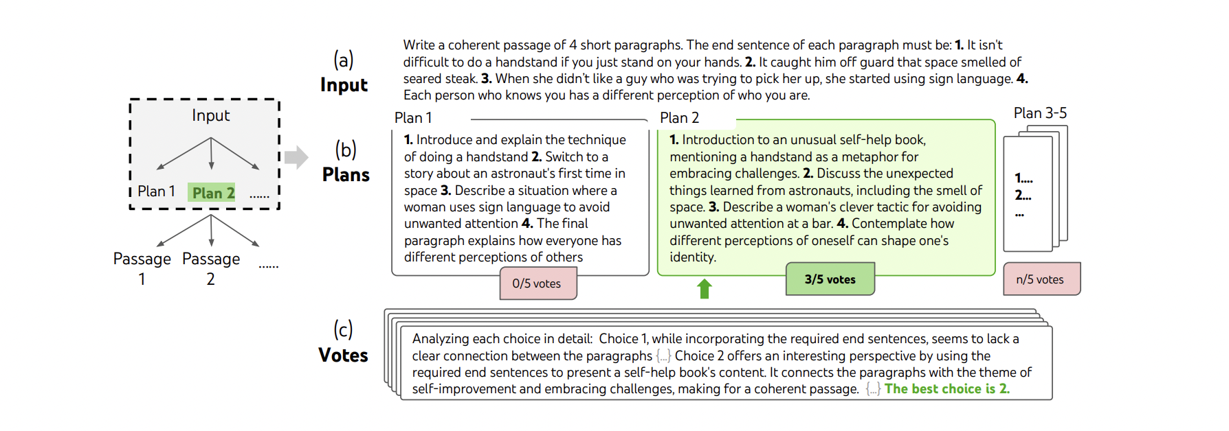 A step of deliberate search in a randomly picked Creative Writing task. Given the input, the LM samples 5 different plans, then votes 5 times to decide which plan is best. The majority choice is used to consequently write the output passage with the same sample-vote procedure.
ToT can substantially outperform simple sampling methods, but it requires more resources and effort to implement. Although, the modular flexibility of ToT allows users to customize such performance-cost tradeoffs.
Parameter Efficient Fine-Tuning
Smart prompting is an important tool, but it doesn’t help when the model has not learned how to solve the problems that will be given to it. A huge performance gains over using the pretrained LLMs out-of-the-box can be achieved via fine-tuning on downstream tasks. However, training the entire model, which has billions of parameters, is computationally expensive and time-consuming, not to mention impossible on most consumer hardware.
This is where Parameter-Efficient Fine-tuning (PEFT) comes in handy. PEFT approaches only fine-tune a small number of (extra) model parameters while freezing most parameters of the pretrained LLMs, thereby greatly decreasing the computational and storage costs.
Prompt-tuning
Prompt-tuning (Lester et al. 2021) is a simple mechanism, which allows to condition frozen LLM to perform specific downstream task. The idea is to prepend different trainable tensors $\mathbf{P_\theta}$ (so called soft prompts) to input embeddings per each task. Unlike the discrete text prompts, soft prompts do not tie to any embeddings associated with the real words and thus they are more expressive for steering the context.
1
2
3
4
5
6
import jax.numpy as jnp

def prompt_tuned_model(token_ids):
    x = embedding(token_ids)
    x = jnp.concatenate([soft_prompt, x])
    return model(x)
Prompt-tuning only requires storing a small task-specific prompt for each task, and enables mixed-task inference using the original pretrained model. Experiments have shown that for large models prompt-tuning produces competitive results as model fine-tuning and its efficiency grows with model size. Also with learned task-specific parameters, prompt-tuning achieves better resilience on domain shift problems. In addition, authors showed that prompt ensembling of multiple prompts beats or matches singular prompts.
Overall soft prompts are incredibly parameter-efficient at the cost of inference overhead (given the quadratic complexity of transformer) and more applicable to larger models (> 10B).
Prefix-tuning
In prefix-tuning (Li & Liang 2021) instead of adding a soft prompt to the model input, trainable embeddings are prepended to the hidden states of all transformer layers. In practice, directly updating $\mathbf{P_\theta}$ leads to unstable optimization and poor performance. To reduce the difficulty associated with high dimensionality training, the matrix $\mathbf{P_\theta}$ is reparameterized by a smaller matrix $\mathbf{P_\theta’}$ composed with a large linear layer $\mathbf{W}$:
\[\mathbf{P_\theta} = \mathbf{P_\theta' W}.\]1
2
3
4
5
6
def prefix_tuned_model(token_ids):
x = embedding(token_ids)
p = soft_prompt @ W
for block in transformer_blocks:
x = block(jnp.concatenate([p, x]))
return x
Prompt-tuning (left) vs prefix-tuning. Note that after training, only $\mathbf{P_\theta}$ is needed for inference, and tensor $\mathbf{W}$ can be discarded.
LoRA
Low-Rank Adaptation (LoRA) (Hu et. al 2021) freezes the pretrained model weights and injects trainable rank decomposition matrices into each layer of the transformer architecture, greatly reducing the number of trainable parameters for downstream tasks. The core idea is to modify linear transformation of input vector $x$
\[h = x\mathbf{W},\]parameterized with a pretrained weight matrix $\mathbf{W}$, with an additional parameter update $\Delta \mathbf{W}$, which can be decomposed into a product of two low-rank matrices:
\[h \leftarrow h + x \Delta\mathbf{W} = x(\mathbf{W} + \Delta \mathbf{W})=x\mathbf{W}+x\mathbf{W_d W_u}.\]Here $\mathbf{W_d} \in \mathbb{R}^{d \times r}$ is down-projection, $\mathbf{W_u} \in \mathbb{R}^{r \times k}$ is up-projection and $r \ll \min(d, k)$ is a bottleneck dimension.
Low rank adaptation. Frozen layers are marked with ❄.
1
2
3
4
def linear_with_lora(x):
    h = x @ W # regular linear
    h += x @ W_d @ W_u # low-rank update
    return h
In the paper experiments LoRA performs competitively even with a very small $r$, such as 1 or 2. Also applying LoRA to both $\mathbf{W}^Q$ and $\mathbf{W}^V$ gives the best performance overall, while adapting only $\mathbf{W}^Q$ or $\mathbf{W}^K$ results in significantly lower performance, even with larger value of $r$.
In general, LoRA possesses several key advantages:
- Low storage requirements. A pre-trained model can be shared and used to build many small LoRA modules for different tasks. We can efficiently switch between tasks by replacing the matrices $\mathbf{W_u}$ and $\mathbf{W_d}$, while keeping base model frozen. This reduces the storage requirement and task-switching overhead significantly.
- Training efficiency. LoRA makes training more efficient and lowers the hardware barrier to entry, since it is not needed to calculate the gradients or maintain the optimizer states for frozen parameters. Instead, only the injected, much smaller low-rank matrices are optimized.
- Inference speed. Simple linear design allows to deploy model with merged trainable matrices and frozen weights: $\mathbf{W} \leftarrow \mathbf{W} + \Delta \mathbf{W},$ thus introducing no inference latency by construction.
- Orthogonality. The combination of LoRA and prefix-tuning significantly outperforms both methods applied separately on WikiSQL benchmark, which indicates that LoRA is somewhat orthogonal to prefix-tuning.
Interestingly, studying the relationship between $\Delta \mathbf{W}$ and $\mathbf{W}$ authors concluded that the low-rank adaptation matrix potentially amplifies the important features for specific downstream tasks that were learned but not emphasized in the general pre-training model. Such statement suggests that LoRA can be applied to RLHF fine-tuning stage, which according to OpenAI is required to “unlock” model capabilities it has already learned.
Adapter
Houlsby et al. (2019) proposed to modify transformer block with additional FFN layers, called (series) adapters. The adapter module is added twice to each transformer layer: after the projection following multi-head attention and after the two feed-forward layers. But like in LoRA, the adapter consists of a bottleneck which has smaller hidden dimension than the input and therefore contains fewer parameters relative to the attention and feed-forward layers in the original model.
Adapter transformation of vector $\mathbf{h}$ can be described as
\[h \leftarrow h + f(h\mathbf{W_d})\mathbf{W_u},\]where $f(\cdot)$ is a nonlinear activation function, e.g. ReLU.
Architecture of the adapter module and its integration with the transformer block.
1
2
3
4
5
6
7
8
def transformer_block_with_adapter(x):
    h = self_attention(x)
    h = h + ffn(h) # adapter
    x = layer_norm(x + h)
    h = ffn(x) # transformer FFN
    h = h + ffn(h) # adapter
    h = layer_norm(x + h)
    return h
Adapter tuning is highly parameter-efficient: training with adapters of sizes 0.5-5% of the original model produces strong performance, comparable to full fine-tuning. In addition to that, Lin et al. (2020) and Pfeiffer et al. (2021) proposed a more efficient design with the adapter layer applied only after the FFN “Add & Norm” sub-layer, which achieves similar performance as using two adapters per transformer block.
MAM adapter
Mix-and-match (MAM) adapter was proposed in a paper by He et al. (2022), where adapter placement and combinations with soft prompts were studied. They measured the performance of all prior methods on four different downstream tasks (summarization, translation, entailment/contradiction and classification), where they also included comparisons with parralel adapters.
Parallel adapters.
They also considered scaling adapter output with tunable parameter $s$. Changing $s$ is roughly the same as changing the learning rate for adapter block if we scale the initialization appropriately. Experiments have shown that scaled parallel adapters outperform series adapters and that placing an adapter in parallel to FFN outperforms adapters parallel to multi-head attention. Finally, they propose MAM adapter, which is a combination of scaled parallel adapter for FFN layer and soft prompt.
1
2
3
4
5
6
7
8
def transformer_block_with_mam(x):
    x = jnp.concatenate([soft_prompt, x])
    h = self_attention(x)
    x = layer_norm(x + h)
    h1 = ffn(x) # transformer FFN
    h2 = scale * ffn(x) # MAM adapter
    h = layer_norm(x + h1 + h2)
    return h
(IA)³
Liu et al. (2022) proposed another PEFT technique, called (IA)³, which stands for “Infused Adapter by Inhibiting and Amplifying Inner Activations”. (IA)³ introduces new parameters $l_v$ and $l_k$, which rescale key and value in attention mechanism:
\[\operatorname{Attention}(\mathbf{Q}, \mathbf{K}, \mathbf{V}) =\operatorname{softmax} \bigg( \frac{\mathbf{Q} (l_k \odot \mathbf{K}^T)}{\sqrt{d_k}} \bigg) \cdot (l_v \odot \mathbf{V}),\]and $l_{ff}$, which rescales hidden FFN activations:
\[\operatorname{FFN}(x) = (l_{ff} \odot f(x\mathbf{W}_1))\mathbf{W}_2\]where $f$ is a nonlinearity activation function. Authors also experimented with T0 model, a variant of famous T5 model by Google, adding auxiliary loss terms to discourage the model from predicting tokens from incorrect target sequences. The called their training pipeline “T-Few” recipe.
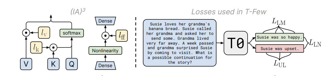 Diagram of (IA)³ and the loss terms used in the T-Few recipe. Left: (IA)³ introduces the learned vectors $l_k$, $l_v$, and $l_{ff}$ which respectively rescale (via element-wise multiplication, visualized as $\odot$) the keys and values in attention mechanisms and the inner activations in position-wise feed-forward networks. Right: In addition to a standard cross-entropy loss $L_{LM}$, an unlikelihood loss $L_{UL}$ and length-normalized loss $L_{LN}$ are introduced. Former lowers the probability of incorrect outputs while latter applies a standard softmax cross-entropy loss to length-normalized log-probabilities of all output choices.
1
2
3
4
5
6
7
8
9
10
11
12
13
14
15
16
17
18
def scaled_self_attention(x):
    k, q, v = x @ W_k, x @ W_q, x @ W_v
    k = l_k * k
    v = l_v * v
    return softmax(q @ k.T) @ V

def scaled_ffn(x):
    x = x @ W_1
    x = l_ff * f(x) # f is nonlinear activation
    x = x @ W_2
    return x

def transformer_block_with_ia3(x):
    h = scaled_self_attention(x)
    x = layer_norm(x + h)
    h = scaled_ffn(x)
    h = layer_norm(x + h)
    return h
(IA)³ adds smaller overhead compared to adapter methods as scale vectors $l_v$ and $l_k$ can be merged into $\mathbf{W}^V$ and $\mathbf{W}^K$ respectively, thus leaving the only overhead from $l_{ff}$. With minimal number of training parameters it achieves comparable results with LoRA and outperforms prompt- and prefix-tuning methods on multiple benchmarks.
Providing external knowledge
Language models show remarkable abilities to solve new problems with just a few examples or textual instructions. At the same time, they struggle with basic functionality, such as arithmetic or factual lookup, where they are outperformed by much simpler and smaller models. They are also unable to solve tasks that require access to changing or private data that was unavailable at training time. To be able to do that LLM must be augmented with additional tools that can provide an external information.
Internet-augmented language models
Lazaridou et. al (2022) proposed to use few-shot prompting to condition LMs on information returned from a broad and constantly updated knowledge source, for example, Google Search. Such approach does not involve fine-tuning or learning additional parameters, thus making it applicable to any language model.
Given a query $q$, clean text is extracted out of multiple URLs returned by search, resulting in a set of documents. Each document is split into $m$ paragraphs $(\mathcal{P})_m$, which are ranked by TF-IDF cosine similarity with a query. Top $n$ paragraphs are selected and each one is inserted separately into the following $k$-shot prompt as the last Evidence:
1
2
3
4
5
6
7
8
9
Evidence: ...
Question: ...
Answer: ...

... (k times)

Evidence: Paragraph
Question: Query
Answer:
This produces $n$ candidate answers $(a)_n$, which can be re-ranked with conditional probabilities $\pi(a \mid q, \mathcal{P})$ and $\pi(q \mid \mathcal{P})$, measured by language model and TF-IDF scores.
 Schematic representation of Internet-augmented LM
TALM
Tool Augmented Language Model (TALM) Parisi et al. 2022 is a LLM augmented with text-to-text API calls. It learns two subtasks at the same time: calling a tool and generating an answer based on tool results.
Tool Augmented LMs.
TALM is guided to generate a tool call and tool input text conditioned on the task input text and invokes a tool’s API by generating a delimiter, such as |result. Whenever this delimiter is detected, the tool API is called and its result appended to the text sequence. TALM then continues to generate the final task output, following |output token:
Input text
|tool-call tool input text
|result tool output text
|output Output text
A weather task example:
How hot will it get in NYC today?
|weather lookup region=NYC
|result precipitation chance: 10, high temp: 20°C, low-temp: 12°C
|output Today’s high will be 20°C
To train TALM authors propose to iteratively fine-tune model on a dataset of tool use examples. Each round model interacts with a tool, then expands the dataset based on whether a newly added tool can improve the generated outputs. Such technique helps to boost the model performance on knowledge and reasoning tasks drastically.
Toolformer
Toolformer (Schick et al. 2023) approach is similar to TALM in that they both aimed for LLMs to teach themselves how to use external tools via simple APIs. Toolformer is trained as follows:
- Sample API calls. First, we annotate a dataset with API call usage examples. It can be done by prompting a pre-trained LM via few-shot learning. An exemplary prompt to generate API calls:
Your task is to add calls to a Question Answering API to a piece of text.
The questions should help you get information required to complete the text. You
can call the API by writing "[QA(question)]" where "question" is the question you
want to ask. Here are some examples of API calls:

Input: Joe Biden was born in Scranton, Pennsylvania.
Output: Joe Biden was born in [QA("Where was Joe Biden born?")] Scranton, [QA("In
which state is Scranton?")] Pennsylvania.

Input: Coca-Cola, or Coke, is a carbonated soft drink manufactured by
the Coca-Cola Company.
Output: Coca-Cola, or [QA("What other name is Coca-Cola known by?")] Coke, is
a carbonated soft drink manufactured by [QA("Who manufactures Coca-Cola?")]
the Coca-Cola Company.

Input: x
Output:- Execute API calls to obtain the corresponding results. The response for each API call $c_i$ needs to be a single text sequence $r_i$.
- Filter annotations based on whether API calls help model predict future tokens. Let $i$ be the position of the API call $c_i$ in the sequence $(x_1, \dots x_n)$ and let $r_i$ be the response from the API. Let also
be a weighted cross-entropy loss with condition $\mathbf{z}$, given as a prefix. Then to decide which API calls are actually helpful, we compare the difference of losses $L_i^- - L_i^+$ to some threshold, where
\[\begin{aligned} L_i^+ &= L_i(c_i \rightarrow r_i),\\ L_i^- &= \min(L_i(\varepsilon), L_i(c_i \rightarrow \varepsilon)) \end{aligned}\]and $\varepsilon$ is an empty sequence. Only API calls with $L_i^- - L_i^+$ larger than some threshold are kept.
- Fine-tune LM on this annotated dataset.
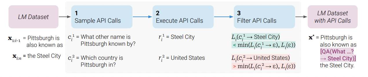 Key steps in Toolformer approach, illustrated for a question answering tool: Given an input text $x$, we first sample a position $i$ and corresponding API call candidates $c_i^1, c_i^2, \dots, c_i^k$. We then execute these API calls and filter out all calls which do not reduce the loss $L_i$ over the next tokens. All remaining API calls are interleaved with the original text, resulting in a new text $x^\ast$.
At inference time, decoding runs until the model produces “$\rightarrow$” token, indicating that it is expecting response from an API call next. At this point, the decoding process is interrupted, the appropriate API is called to get a response, and the decoding process continues after inserting the response.
Toolformer considerably improves zero-shot performance of language model, e.g. augmented GPT-J (6.3B) even outperformed a much larger GPT-3 model on a range of different downstream tasks.
Conclusion
The list of techniques in this post is far from complete, but it provides direction for those who are looking for a way to make their language model more useful. Assistants based on Large Language Models are relatively new and, while extremely powerful, still face many limitations that can be worked around in a variety of ways. It is only a matter of time before language models cease to be used for entertainment purposes and enter our daily lives as a complete and useful tool.
A similar idea but with use of reinforcement learning instead of tree search was proposed by Long (2023). ↩