Applying Graph Neural Networks to Kaggle Competition

Few months ago, Kaggle launched featured simulation competition Kore-2022. In this kind of competitions participants bots are competing against each other in an game environment, supported by Kaggle. Often there are 2 or 4 players in a game, at the end each winner/loser moves up/down according to skill rating system. Team reaching top-rating wins.

Kore rules

That’s how entry to Kore competition looks like:

In this turn-based simulation game you control a small armada of spaceships. As you mine the rare mineral “kore” from the depths of space, you teleport it back to your homeworld. But it turns out you aren’t the only civilization with this goal. In each game two players will compete to collect the most kore from the board. Whoever has the largest kore cache by the end of 400 turns—or eliminates all of their opponents from the board before that—will be the winner!

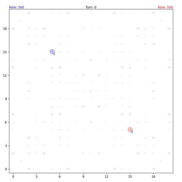Fig. 1. Gameplay visualization by Tong Hui Kang

Game setup looks extremely complex at first glance (at least compared to the other Kaggle simulation competitions like Hungry Geese, which was basically a variation of Tetris Snake game).

Here I’ll try to list the main rules:

• The game board is 21x21 tiles large and wraps around on both the north/south and east/west borders
• You start the game with 1 shipyard and 500 kore.
• Each turn you can either spawn new ships (each costs 10 kore), or launch fleet with a flight plan, or do nothing.
• Flight plan is a sequence of letters and integers:
  • ‘N’, ‘E’, ‘S’ or ‘W’ defines the direction of the fleet.
  • The integer following the letter determines how many steps (+1) fleet will take in that direction.
  • For example, ‘NE2SW’ forms a circle trajectory, where fleet makes one step up, three steps right, one step down and then it moves left until it reaches starting point.

  • The maximum length of the flight plan depends on fleet size by formula:

    \[\max \text{length} = \lfloor 2 \log(\text{fleet size}) \rfloor + 1\]

    E.g. the minimum number of ships for a fleet that can complete a circle like ‘NE2SW’ is 8.

  • If plan ends with ‘C’, at the end tile of the flight fleet builds a shipyard, consuming 50 of its ships.
• Each fleet does damage to all enemy fleets orthogonally adjacent to it equal to its current ship count. Destroyed fleets drop 50% of their kore onto their currently occupied position with 50% being awarded to their attackers. If the attacking fleet does not survive, the kore is dropped back onto the tile instead.
• Fleets that move onto the same square collide. Allied fleets are absorbed into the largest fleet. The largest fleet survives and all other fleets will be destroyed. The remaining fleet loses ships equal to the ship count of the second largest fleet. The largest fleet steals all of the kore from other fleets it collides with.

In a nutshell: you collect kore, spawn ships and try to destroy all of enemy objects before he destroys yours. The main difficulty for player is to construct an optimal path planning solution for fleet flights. Players must calculate many steps ahead as the effects of their actions in most cases do not appear immediately.

Graph construction

Now how one can approach this task? Prior to this competition, Kaggle launched its trial version, Kore Beta, with the only difference being that it was 4-players game. First places were taken by rule-based agents, based mostly on simple heuristics.

Another way is to think of this task as text generation. One can train a network which takes board image as input and returns flight plan as text output for each shipyard. A solution with this kind of approach took one of the top places eventually.

One can also represent board as graph, where each tile is a node and edges connect adjacent tiles. Then each turn, when a fleet is sent from shipyard, searching for optimal flight plan is equivalent to searching for optimal path on a graph.

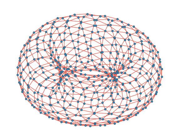Fig. 2. This is how periodic 21x21 grid looks like: a doughnut.

One of the main advantages of an algorithm on a graph is rotation equivariance. Board is symmetric, therefore algorithm behaviour must not change if we swap players initial positions. With standard convolutional networks we can try to overcome this issue by using augmentations, but there is no need for them if we use graph neural networks.

We also don’t want to miss the information which is not included in this kind of board representation: future positions of fleets. We know all of them by fact, because players plans are not hidden from each other. Therefore, it seems useful to add board representations at the next step, at the step after next and so on until we reach desirable amount of steps. Also, after we make our moves, these future graphs may change, so it doesn’t always seem reasonable to look far away from current step. In my implementation I was looking 12 steps ahead.

Fig. 3. Graph zoomed in. Each node corresponds to a tile on the board, each edge represents that either nodes are spatial neighbors, or they are the same tiles but at adjacent timestamps. Graph is oriented, nodes from future graphs are pointing at nodes at previous steps. Thus, all the information flows to current board representation which will be used for actions generation later.

Node input features $\mathbf{v}_i$ contain kore amount on the tile, timestamp, total amount of kore collected by player and its opponent. Also, if any fleet is located on the tile - its cargo, collection rate and number of ships. If any shipyard is on the tile - its number of ships, maximum plan length for this number and maximum number of ships, which can be spawned.

The edge input features $\mathbf{e}_{ji}$ are $(1, 0, 0)^T$, $(0, 1, 0)^T$ and $(0, 0, 1)^T$ for temporal, lateral and longitudinal edges respectively. Basically, they are one-hot representations of these edge classes. Why treat spatial edges differently? When you create a flight plan, its length increases when fleet makes a turn: while for both “N1S” and “NEWS” fleet moves 2 tiles from shipyard and returns back, the first one is smaller and requires fewer ships.

Graph Encoder Architecture

If we had to work with standard representations of board, we would most likely use convolutional layers. There exists an analogue of convolutions in a graph world, called, big surprise, graph convolutions. Similarly to ResNet architecture we can build a ResGCN encoder:

Fig. 4. Bird’s eye view of graph encoder architecture. The summation of ResGCN input and output graphs is performed both over node and over edge features.

It is also extremely important to make our graph neural network anisotropic, which means that each neighbor should have a different effect on the node depending on the weight of the edge between them. The idea is that the neural network transforms the nodes in such a way that the encoded features of the nodes lying on the agent’s path are more similar to each other than to nodes that are not.

Fig. 5. ResGCN architecture. First, node features are encoded through several independent ResGCN blocks. Each block is a mapping $\mathbb{R}^d \rightarrow \mathbb{R}^{d/n}$, where $n$ is a number of blocks. Outputs are concatenated together, constructing vector of the same size as the input. Then to get new edge features we pass outputs through feed-forward layers: $\operatorname{Query}, \operatorname{Key} \in \mathbb{R}^{d \times 3}$, followed by element-wise multiplication and $\operatorname{tanh}$ activation.

ResGCN block consists of sequential graph convolutional layers:

\[\operatorname{GCN}(v_i, e) = \Theta^T \sum_{j\in\mathcal{N}(i) \cup \lbrace i \rbrace} \frac{e_{ji}}{\sqrt{\hat{d}_i \hat{d}_j}} v_j\]

with \(\hat{d}_i = 1 + \sum_{j \in \mathcal{N}(i)}e_{ji}\) and $\mathcal{N}(i)$ - set of all neighbors for node $v_i$.

Fig. 6. ResGCN block schema. GraphNorm layer normalizes node features over each graph in a batch.

Imitation learning

Now, we can train our network to imitate actions of best agents on a leaderboard. Each turn for each node with player shipyard on it, we have to decide for two things:

• Should we spawn, launch or do nothing?
• What is a number of ships to be spawned/launched?

One can train a network with cross-entropy loss for the action and mean-squared loss for the ships number. However, due to the fact that flight plan length depends on discretized $2 \log$ of fleet size, we can end up with errors like predicting number of ships to be $20$ with true number $21$ and thus having maximum plan length of $6.99$ and not being able to build a path with desired length of $7$. To avoid this we must split our policy into multiple classes, each representing maximum flight plan length:

• Do nothing
• Spawn
• Launch 1 ship (maximum length 1)
• Launch 2 ships (maximum length 2)
• Launch 3 or 4 ships (maximum length 3)
• …
• Launch 666, 667, …, 1096 ships (maximum length 14)

Here in total we have 16 classes, but this amount can be reduced or increased, depending on what engineer thinks is a reasonable number. To choose a fleet size we can set our target to be a ratio of ships to total amount of ships in a shipyard (or to maximum spawn number in case of ‘spawn’ action).

Fig. 7. Main policy heads. Encoded embedding is taken from node of current board graph representation, where shipyard is located on. This embedding is passed through linear layer to predict an expert action. In parallel, it is concatenated with one-hot representation of expert action and then goes through another feed-forward layers to predict expert spawn/launch ships ratio. On inference, $\arg\max$ of agent predictions can be used instead of expert action.

Finally, we face path generation task. The idea is that for each node, starting from shipyard, we take all of its neighbors and itself, and predict next node in a flight plan. If it chooses node itself, we convert ships to a new shipyard (we can mask such action if fleet size is less than 50 or if fleet is already on a shipyard). To make the prediction dependent not only on the current node, but also on the entire sequence of previously selected nodes, we can use recurrent layers. It is also important to consider amount of space we have left for path generation.

Fig. 8. Path policy head. We start at shipyard node. At each step all neighbor candidates, including node itself, are concatenated with one-hot representation of a ‘space left’ for plan generation. Then they are passed through recurrent layer. Received neighbor embeddings are passed through linear layer $\operatorname{Query}$ and multiplied with node features passed through $\operatorname{Key}$ layer. Resulting vector represents probabilities of each neighbor to be the next node. Then we move along path defined by an expert agent and repeat the same procedure.

Now having probabilities for each move, we can generate path by greedy or beam search, cutting path when it reaches shipyard or when there is no more space left. There is also a case, when path stuck in a loop like ‘NW999..’, and it can take forever until we won’t have enough space. For such thing it is useful to make a stop by some maximum-moves threshold.

Bonus: reinforcement learning

In my experiments, imitation learning was good enough for an agent to start making good moves, however, there was constant instability on inference. At some point an agent could make a ridiculously stupid move (with small probability, but nevertheless), effecting balance of the game dramatically. This move could’ve never been made by an expert agent, therefore we end up with board state which neural network didn’t see in training data. So the chance of making wrong moves increases at each step and finally imitation agent loses.

To tackle this issue I’ve tried off-policy reinforcement learning. The architecture of policy neural network was the same, critic neural network had similar but smaller encoder. Reward was +1 for winning, -1 for losing. I used TD($\lambda$) target $v_s$ for value prediction and policy loss with clipped importance sampling:

\[\mathcal{L}_{value} = (v_s - V_\omega(s))^2, \quad \mathcal{L}_{policy} = -\log \pi_\theta(a|s) \min \big(1, \frac{\pi_\theta(a|s)}{\beta(a|s)} \big) A_\omega(a, s),\]

where $A_\omega(a, s)$ is an advantage, obtained by UPGO method.

RL helped to stabilize inference, but sadly it didn’t go far beyond that. New agent was able to beat rule-based agents, which were on top of Kore Beta competition ~80% of the time.

Results and conclusions

Unfortunately, best of my agents were able to reach only up to 30-ish places, but still, it was a fun ride. What could’ve been done better? Here is my list:

• Better feature engineering. The input state which I was using contained a lot of data, however not all of the important information could have been distilled by neural network. Looking ahead for 12 steps made input graph enormously huge: $21 \times 21 \times 12 \times n$, where $n$ is a feature dimension for every node. And still there were a lot of opponent flight plans with bigger time-length than 12 steps.
• Larger neural network. It is related to previous issue: construction of huge input state at every turn was taking a lot of time on inference. In order to fit Kaggle time requirements I had to reduce network size. I’m convinced that bigger dimensions could lead to better results.
• Reinforcement learning experiments. It is well known that it takes a lot of time to make RL work. Training is slow and unstable most of the time. It is extremely important to closely monitor training procedure and analyze the results.

Hopefully I’ll take this experience into account in the next Kaggle simulation competition.